Writing Your First Python Code

To begin coding, open your test.py file and enter the following code:

print("Hello World!")

Next, hit the Run or Play button in your IDE. This will execute the code, and the terminal should pop up, displaying your message:

Hello World!

Look at you—your very first line of code!
Too easy, right? And the best part is, you can change the text inside the quotes to say anything you want. For example:

print("Veni, Vidi, Vici")

Go ahead—try it out!

Why We Use Packages in Python

Code is always written with a purpose—to calculate a company’s revenue, visualize data with beautiful graphs, or even build immersive virtual worlds. But here’s a question:
What happens when two people want to achieve the same goal?
Should they both write the exact same code from scratch? That wouldn’t make much sense, right?

That’s where packages (also referred to as libraries) come in.

A package is a collection of code that someone else has already written, tested, and documented—so you don’t have to reinvent the wheel. Each package usually comes with a documentation file: a list of available functions and a description of what each one does.

For example, a math package might include functions for:

• Addition
• Multiplication
• Calculating derivatives
• And much more

Let’s say you’re building a calculator. You’ve written everything yourself, but you don’t feel like coding a derivative function from scratch. Instead, you search for a package that already does that.
You read its documentation, install it, and then import it into your project.

To do that, Python uses something called an API (Application Programming Interface). Think of an API as a bridge between your code and someone else’s code (the package). You don’t need to understand how the package works internally—you just use its functions through the API.

Now, when you share your project, others will also need access to the same packages you used. These are called dependencies. If your project depends on a package, and that package depends on another, all of them need to be installed for your code to run correctly.

Packages in This Course

In this course, you’ll build key machine learning algorithms from scratch—which means we’ll implement the actual logic ourselves. However, for things outside the core focus of the course—like matrix math, data loading, or plotting graphs—we’ll use existing packages to save time and effort.

This allows us to focus on the concepts that matter most, without getting bogged down in boilerplate code.

Installing Your First Package: numpy

Let’s start by installing a popular package called NumPy, which is used for scientific computing in Python.

1. Open the terminal in your IDE. For Pycharm: Press the cube with the code symbol on the left side bar. For Visual Studio Code: Press “Terminal” then “New Terminal” on the top bar.
2. Type the following command and press Enter:

pip install numpy

If you wanted to install a different package, you’d simply replace numpy with that package’s name. Your IDE usually handles any extra dependencies automatically, so you don’t need to worry about it.

Importing the Package in Your Code

After installation, open your test.py file and add this line on the top of the page:

import numpy as np

The as np part is just a shortcut. It allows us to use np instead of typing out numpy every time we use one of its functions. You can also remove it if you prefer it that way.
(Programmers are famously efficient—or just lazy, depending on how you look at it.)

As a general rule, all import statements should be placed at the very top of your Python file.

Using The Numpy API

Now that we’ve imported the NumPy package, let’s actually put it to use. To call any function from NumPy, just write np.FUNCTION_NAME(), replacing FUNCTION_NAME with the method you want to use. (Also, make sure you understand what type of input this method expects and the correct order in which to provide it.)

If you’re curious to see what cool things NumPy can do, check out the official documentation:

NumPy Documentation

Let’s start with a simple example:

import numpy as np


a = 10
b = 20

result = np.add(a, b)

print(result)

The output will be:

30

Here, we used the add() function from NumPy’s API by typing np.add(). That’s really all an API is—it acts as a bridge between your code and the tools NumPy offers. You don’t need to know exactly how add() works under the hood to benefit from it. You just use it and move on.

What are Arrays?

Obviously, NumPy is not just used for addition. It can do a lot more powerful things, which you’ll see throughout this course. One of its strongest features is the ability to create n-dimensional arrays and use them in all sorts of calculations.

In computer programming, an array is a data structure used to store and access a collection of values. You can think of an array as a row of boxes, where each box holds a specific value or number.

A 1D (one dimensional) array might look like this:

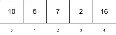
Now, let’s say you want to access the number 2. You don’t ask the computer directly for the value 2; instead, you ask:
“What’s inside box number 3?”

In programming, this process is called indexing. And here’s something important:
Computers start counting from 0, not 1. So in the example above:

• Box 0 contains 10
• Box 1 contains 5
• Box 2 contains 7 and so on.

If you wanted to change the value in box 3, you could simply overwrite it.

Now let’s take it one step further with a 2D array:

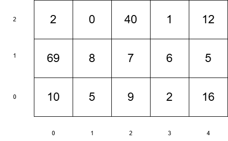
To access a value now, you need two indices:

• The first tells you the row
• The second tells you the column

Think of it like a coordinate system, and yes—both indices start at 0.

Let us go even beyond 2D. A 3D array would look like this:

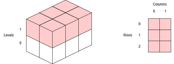
Think of it as a cube, where each Level of the cube represents the 2D array from above. Now, you have three indices to work with: one for the level, one for the row, and one for the column (In this order). And as you’d expect, they all start from 0.

Working with Arrays in NumPy

Let’s look at how we can create arrays using NumPy.

Creating a Simple Array (1D)

Here’s how you create one:

import numpy as np


array = np.array([1, 2, 3, 4, 5])

print(array)

Output:

[1,2,3,4,5]

You just created a 1-dimensional array with 5 elements.

Creating a 2D Array

import numpy as np


array_2d = np.array([[1, 2, 3], [4, 5, 6]])

print(array_2d)

Output:

[[1 2 3]
 [4 5 6]]

This is a 2×3 array — 2 rows and 3 columns.

Creating Higher-Dimensional Arrays

You can go higher. For example, a 3D array looks like this:

import numpy as np


array_3d = np.array([
  [[1, 2], [3, 4]],
  [[5, 6], [7, 8]]
])

print(array_3d)

Output:

[[[1 2]
  [3 4]]

 [[5 6]
  [7 8]]]

It’s difficult to visualize arrays with more than three dimensions using a simple print statement. That’s why we rely on the size and shape of arrays to understand their structure.

Indexing Arrays in NumPy

You can index elements in an array using square brackets like this: (index 0)

import numpy as np


array = np.array([1, 2, 3, 4, 5])

print(array[0])

Output:

1

For a 2D array, indexing works like this: first rows, then columns. (row 0 and column 1)

import numpy as np


array_2d = np.array([[1, 2, 3], [4, 5, 6]])

print(array_2d[0][1])

Output:

2

For a 3D array, the process is the same, but you use three indices—one for each dimension—inside three sets of brackets. As a helpful tip: The last bracket corresponds to the columns, while the second-to-last one refers to the rows. With this in mind, you’ll have a clearer understanding of the structure, regardless of the array’s dimensions.

Slicing in NumPy

Do you want to know what blew my mind when I first saw it? THIS!

import numpy as np


array = np.array([1, 2, 3, 4, 5])

print(array[1:3])

Output:

[2 3]

You can easily access a specific range of numbers using the colon : symbol, inside of the index bracket, which represents a range from x to y. For example, “give me the boxes from box 2 to 4” is achieved with slicing. It’s called slicing because you’re essentially “cutting” parts of the array. How awesome is that? In Java, I’d need to write several lines of code to achieve the same thing, but here, it’s as simple as using a colon. It honestly feels almost too easy sometimes.

This also works with 2D arrays (and with any n-dim. array):

import numpy as np


array_2d = np.array([[1, 2, 3], [4, 5, 6]])

print(array_2d[0:1][0:])

Output:

[[1 2 3]]

By writing just 0:, you’re telling the program to start at index 0 and take all the remaining elements from that point onward. It’s a simple and efficient way to grab everything after the first element. It works the other way around too. Using :5 means “take every element up to, but not including, index 5.”

Checking the Size and Dimensions of a NumPy Array

Throughout this course, we’ll be working extensively with arrays like these. There will be times when we don’t define them manually, but instead receive them from other sources—such as when importing a dataset. In these situations, it’s helpful to know the size (the total number of elements in the array) or the shape (its dimensional structure), so you can adjust your code accordingly or pinpoint potential sources of errors or bugs.

Each NumPy array—your actual array object—comes with a variety of built-in attributes and functions that you can access directly, without needing to call them through np.FUNCTION_NAME().

An attribute of an object (in this case, your array) is something that describes or provides information about the object. For example, the size of the array—the number of elements it contains—is an attribute. To use a real-world analogy: if your object were a car, its color would be an attribute.

Unlike functions, attributes don’t do anything; they simply describe the object. In code, you can easily tell them apart:

Attributes are accessed without parentheses:

# returns the dimensions of that array
your_array.shape

Functions, on the other hand, require parentheses:

# returns the sum of the elements in that array
your_array.sum()

For operations involving multiple arrays, such as addition, it’s common to use functions from the NumPy module directly—for example, np.add(array1, array2) as shown earlier. However, when you’re working with just a single array and want to access specific information—like its shape—you can use the array’s built-in attribute: your_array.shape.

This is equivalent to calling np.shape(your_array), but using the attribute directly is often simpler and more intuitive.

(By the way, when performing arithmetic operations like multiplication, addition, subtraction, and so on, you don’t need to use functions like np.add() every time. Instead, you can simply use the standard arithmetic operators—for example, arr1 + arr2. Just replace the + with the operator you need (-, *, /, etc.) to perform the desired operation directly and more intuitively.)

If you’re wondering what that green line above is—it’s called a comment. In Python, comments start with the # symbol. Anything written after that symbol on the same line is ignored by the computer. Comments are used to explain what the code is doing or to add helpful descriptions for anyone reading it.

Lets look at an example that combines everything we just learned:

import numpy as np

# creating array
array_2d = np.array([[1, 2, 3], [4, 5, 6]])

# let's pretend we do not know the shape and size
print(array_2d.shape)
print(array_2d.size)

# let's call a method on our array
print(array_2d.sum())

Output:

(2, 3)
6
21

In this context, (2, 3) means the array has 2 rows and 3 columns.

If you’re working with a 3D array, like the one shown earlier, a shape of (2, 2, 2) means you have 2 two dimensional arrays, each with 2 rows and 2 columns.

And that’s it! You now know how to create arrays in NumPy, index them, slice them, as well as how to check their size and shape. You’ll use these skills a lot in machine learning, so take a moment to try creating a few of your own arrays and play around with different dimensions.

Tip: Instead of creating arrays manually, use methods like np.random.randint() or np.zeros(). You can easily explore these methods by hovering over them in your IDE to access the documentation. Here’s another handy IDE tip: when you type “np.”, press “Control + Space” to bring up a list of available methods. (If it does not do it automatically)

I won’t be diving into every single detail of NumPy here. Instead, I’ll only cover the parts we need as we go. But if you’re curious and want to explore more of this powerful and beautiful library, you can check out the tutorials available on this site:

NumPy Documentation