What Are Vectors?

That depends on who you ask.

To a physicist, a vector is an arrow in space. It has two key properties: a length, which represents its magnitude (or strength), and a direction, which shows where the force or movement is applied. If two vectors have the same length and direction, they are considered the same—regardless of where they are placed in space. You can move the arrow up, down, or anywhere else, and it remains the same vector.

To a computer scientist, on the other hand, a vector is typically an ordered list of numbers. The word “ordered” is crucial here—\(\begin{bmatrix} 14 \\ 2 \end{bmatrix}\) is not the same as \(\begin{bmatrix} 2 \\ 14 \end{bmatrix}\). Each number in the list often represents a specific feature. For example, in a car dataset, the first entry might indicate the car’s age, and the second the number of previous owners. The length of the list determines the vector’s dimension: two numbers mean a 2D vector, three numbers mean a 3D vector, and so on.

A mathematician takes a more abstract approach. To them, an object is considered a vector if two operations can be performed on it:

1. Vector addition – \(\mathbf{v} + \mathbf{w}\) – combining two vectors to produce a third.
2. Scalar multiplication – \(2 \cdot \mathbf{w}\) -multiplying a vector by a number (a scalar) to produce another vector.

From this general perspective, both the physicist’s and the computer scientist’s interpretations qualify. In fact, even something like a polynomial can be seen as a vector under this broader definition.

We’ll represent vectors using boldface, like \( \mathbf{v} \). You may have seen vectors written with an arrow above the letter, like \( \vec{v} \), especially in school. However, we’ll use bold notation, as it’s more common in both machine learning and advanced mathematics.

In addition, we will represent vectors as elements of \( \mathbb{R}^n \), which simply means they are ordered tuples of \(n\) real numbers, with \(n \in \mathbb{N}\). Here, \(n\) refers to the dimension of the vector. For example:

\(\mathbf{v} = \begin{bmatrix} 1 \\ 2 \\ 3 \end{bmatrix} \in \mathbb{R}^3\)

is a 3-dimensional vector. If we were working in two dimensions, the vector would belong to \(\mathbb{R}^2\)

This representation also satisfies the mathematician’s requirements: When two vectors in \(\mathbb{R}^n\) are added together, the result is still in \(\mathbb{R}^n\). Similarly, multiplying a vector in \(\mathbb{R}^n\) by a real number (a scalar) also produces a vector in \(\mathbb{R}^n\). Another benefit of using \(\mathbb{R}^n\) is its natural alignment with how computers store and handle numerical data—essentially as arrays of real numbers.

If you’re unfamiliar with the symbol \(\mathbb{R}\), it represents the set of all real numbers. In mathematics, different sets are used to classify types of numbers:

• \(\mathbb{N}\): the natural numbers (positive whole numbers like 1, 2, 3…)
• \(\mathbb{Z}\): the set of all integers, including negative numbers (…–3, –2, –1, 0, 1, 2, 3…)
• \(\mathbb{Q}\): the set of rational numbers (numbers that can be expressed as a fraction of two integers, where the denominator (the number under the fraction line) is not zero)
• \(\mathbb{R}\): the set of all real numbers, including both rational and irrational numbers

So, when we say a vector belongs to \(\mathbb{R}^n\), we mean that each of its components is a real number—it could be positive, negative, a fraction, or an irrational number. (We’re excluding complex numbers to keep things straightforward and they aren’t part of the real number set anyway.)

When you hear the term “set,” think of it like a box containing specific items, where each item is unique (no duplicates). If we’re talking about a set of numbers like \(\mathbb{R}\), the items in the box are real numbers. If we’re discussing a set of vectors, the items are vectors.

Moreover, we’ll be talking a lot about vector spaces—but I’ll spare you the formal definition for now. Just imagine a vector space as a structured world where vectors live and interact. For example, in 2D, picture a blank sheet of paper in front of you: every arrow you can draw on that sheet, starting from the origin and pointing in any direction, is a vector. That whole flat plane is their world—the vector space.

In this course, we will also use visual representations of vectors alongside their numerical form. This dual approach helps build a stronger intuition for how vector operations work. Geometrically, you can think of a vector as an arrow that starts at the origin (where the x- and y-axes intersect) and points to a specific location in space. Every vector is associated with a list of numbers that tells us how to construct it. The first number corresponds to movement along the x-axis, the second to the y-axis. For example, the vector \(\begin{bmatrix} 4 \\ 6 \end{bmatrix}\) means you start at the origin, take 4 steps to the right (along x), and 6 steps up (along y). If the numbers are negative, you move in the opposite direction (left or down).

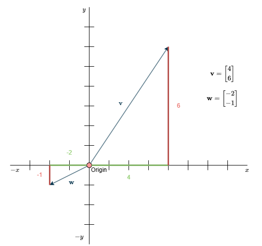
This concept extends to three dimensions as well. A 3D vector like \(\begin{bmatrix} 4 \\ 6 \\ 2 \end{bmatrix}\) includes a third number for the z-axis, which is perpendicular to both the x- and y-axes. This tells us how far to move along the z direction—upward or downward in 3D space.

Each vector has a unique list of numbers, and each list represents one and only one vector.

Vector Addition

The two operations introduced earlier form the foundation of linear algebra—almost everything in this field builds upon them. That’s why it’s essential to understand them thoroughly. Let’s begin with vector addition.

Geometrically, to add two vectors, you place the tail of one vector at the head (tip) of the other. You can also do it in the opposite order—it doesn’t make a difference; the result is the same. Once positioned, draw a new vector from the tail of the first (origin) to the head of the second—this new vector represents their sum.

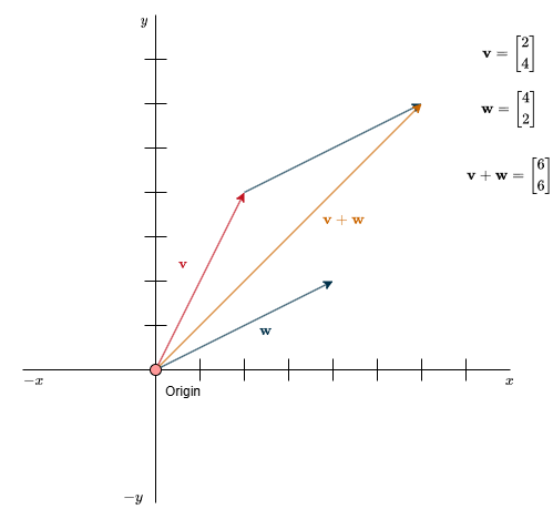
Imagine you’re on a treasure hunt and receive two sets of directions. The first says to move 3 steps right and 2 steps up; the second says to go 1 step right and 4 steps up. You could follow the first set of steps, then the second—or combine them into a single path: 3 + 1 steps to the right and 2 + 4 steps up. Either way, you’ll arrive at the same point.

In this way, each vector can be thought of as a movement or flow in space. Following one vector after another is equivalent to taking a single step along the vector that represents their total combined movement.

Mathematically, vector addition is defined as:

\(\mathbf{v} + \mathbf{w} = \begin{bmatrix} x_v \\ y_v \end{bmatrix} + \begin{bmatrix} x_w \\ y_w \end{bmatrix} = \begin{bmatrix} x_v + x_w \\ y_v + y_w \end{bmatrix}\)

Scaling Vectors

The next operation is multiplying a vector by a number. This number can be any real number. Going back to our direction-instruction analogy: imagine I now tell you to go twice as far as before. You’d correctly assume that you need to double your steps in each direction.

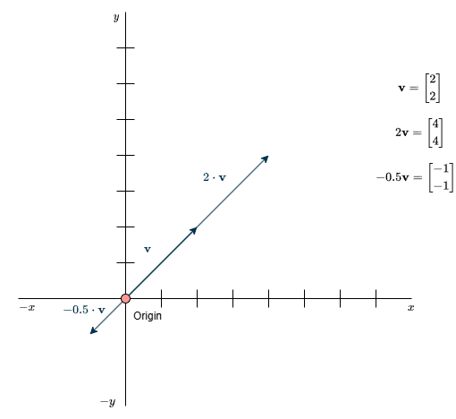
Through this operation, we can make a vector longer, shorter, or even reverse its direction. If we multiply by a negative number, the direction flips—going right becomes going left, and up becomes down. In other words, the vector is mirrored in the opposite direction.

This process of changing a vector’s size or flipping its direction is called scaling, and the number used to do it is called a scalar. I’ve been doing some work in machine learning over the past year and only just realized that’s why a single number is called a scalar—it took me long enough.

In most of linear algebra, numbers are almost always used to scale vectors, so it’s common to see the terms number and scalar used interchangeably.

In mathematical terms, scaling a vector is represented by:

\(c \cdot \mathbf{v} = c \cdot \begin{bmatrix} x \\ y \end{bmatrix} = \begin{bmatrix} c \cdot x \\ c \cdot y \end{bmatrix}\)

with \(c \in \mathbb{R }\)