Null Spaces and Column Spaces

Every linear transformation naturally comes with two important sets of vectors: first, the vectors it sends to zero, essentially the ones it “throws away”, and second, the vectors it actually reaches. These two sets form subspaces known as the null space and the column space, respectively. Understanding them will give us significant problem-solving power.

Functions

Before introducing the new subspaces, let’s briefly review the basic terminology of functions. Suppose we have two sets \(A\) and \(B\). A function from \(A\) to \(B\) is a rule that assigns to each element of \(A\) exactly one element of \(B\). We denote this by

\(f: A \rightarrow B\)

This idea shouldn’t feel unfamiliar, linear transformations are functions, and we have already discussed them. The set \(A\) from which a function takes its inputs is called the domain, and the set \(B\) that contains all possible outputs is called the codomain. A key requirement is that each input has exactly one output. For example, an element \(a_1 \in A\) cannot be mapped to both \(b_1\)​ and \(b_2\) ​at the same time; such ambiguity would violate the definition of a function.

Another way to visualize this is by plotting the relationship between the sets on a graph. Imagine placing the domain on one axis and the codomain on the other. For instance, if both sets are \(\mathbb{R}\), we can represent one along the \(x\)-axis and the other along the \(y\)-axis. A map is a function precisely when it passes the vertical line test: any vertical line should intersect the graph at most once. If a vertical line crosses the graph more than once, the rule assigns multiple outputs to the same input and therefore is not a function. The following curve fails this test:

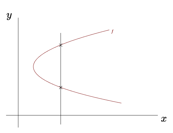
Here is an example of a graph that does pass the vertical line test:

Functions can relate elements of two sets in different ways. Three important properties are injectivity, surjectivity, and bijectivity. Let’s go through them one at a time.

Injectivity

A function is injective (also called one-to-one) if no two different inputs share the same output. In other words, each element of the codomain is mapped to at most once. Formally, a function \(f:A \rightarrow B\) is injective if

\(f(a_1) = f(a_2) \Rightarrow a_1 = a_2\)

It is perfectly fine for some elements of \(B\) to have no incoming arrows (that is, not be hit by the function at all). What matters is that no element in \(B\) is hit twice. The following example is not injective:

Since \(b_2\) receives arrows from two different elements of \(A\). This still satisfies the definition of a function, but it fails the injectivity condition.

Surjectivity

A function is surjective (also called onto) if every element of the codomain is hit by at least one input from the domain. Formally, a function \(f:A \rightarrow B\) is surjective if

\(f(a) = b \;|\; \forall b \in B, \; \forall a \in A\)

In a surjective function, nothing in the codomain is “left out.” Every element of \(B\) must have at least one incoming arrow.

Having multiple incoming arrows is not a problem here, as long as the element is hit at least once. Here is an example of a function that is not surjective:

Since \(b_3\)​ is not hit, it receives no incoming arrows.

Bijectivity

A function is bijective if it is both injective and surjective. This means that each element of \(A\) is mapped to exactly one element of \(B\), and every element of \(B\) is hit by exactly one element of \(A\). In other words, a bijection creates a perfect one-to-one correspondence between the two sets. The figure at the beginning of this section illustrates this idea.

Bijective functions are invertible, they can be “undone.” Because there is a perfect one-to-one correspondence between \(A\) and \(B\), we can simply reverse the arrows. The inverse of a function is denoted by

\(f^{-1}: B \rightarrow A\)

and it reverses the action of \(f\).

This is not possible if the function is only injective or only surjective. If the function is not surjective, some elements of \(B\) have no incoming arrow; reversing the arrows would leave nowhere to go in \(A\). If the function is not injective, some elements of \(B\) have multiple incoming arrows; reversing them would be ambiguous because we wouldn’t know which element of \(A\) to return to. Only bijective functions avoid these problems, which is why they, and only they, have well-defined inverses.

The only thing left to recap is the range of the function.

Range

The range (also called the image of \(f\)) of a function is the set of all actual outputs the function produces. More formally, if

\(f: A \rightarrow B\)

then the range is defined as

\(\text{range}(f) = \{f(a) \; | \; a \in A\} \subseteq B\)

Think of the codomain \(B\) as a city and the function as a radio tower. The range tells you which houses in the city actually receive the signal. In other words, the range is the set of outputs the function truly reaches. For example, consider

\(f: \mathbb{R} \rightarrow \mathbb{R}, \hspace{1cm} f(x) = x^2\)

The codomain is all real numbers, but since squaring never produces a negative value, the function never reaches the negative part of \(\mathbb{R}\). Therefore, the range is only the non-negative real numbers.

Surjectivity guarantees that

\(\text{range}(f) = \text{codomain}(f)\)

because it requires that every element of the codomain be hit by at least one input. Now we’re finally ready to tackle the new subspaces.

Null Space

The definition above says that all the vectors that \(T\) maps to zero are gathered into a single set. This set forms a vector space, and we call it the null space, “null” hinting at the fact that it involves the zero vector. It is also sometimes referred to as the kernel. Consider the following figure:

In this example, the set \( \{ \mathbf{0}, \mathbf{v}_1​,\mathbf{v}_2​, \mathbf{v}_3 \} \) forms the null space of the transformation. Recall that a subset must contain the zero vector to qualify as a subspace. Since every linear transformation satisfies \(T(\mathbf{0}) = \mathbf{0}\), every linear transformation has a null space regardless of its other properties. However, the null space can be larger than the trivial subspace \(\{\mathbf{0}\}\). As soon as it contains a nonzero vector, all scalar multiples of that vector must also lie in the null space, which immediately gives us infinitely many vectors. Note that the null space is a subspace of the input vector space, not the output space. In other words, it’s a subspace of \(V\), it lives in \(\mathbb{R}^n\).

If \(T\) is injective, meaning that every vector in the output space is hit at least once, including the zero vector, then the null space of \(T\) is as small as possible: \(\{\mathbf{0}\}\). Simply put:

injective \(T \Longleftrightarrow\) null space equals \(\{\mathbf{0}\}\)

Notice that this statement works both ways: if the null space is as small as possible, then the transformation is injective. That’s half the story when it comes to checking whether a transformation is invertible. But as soon as there’s even a single nonzero vector in the null space, you can throw invertibility out of your window. Let me make this clearer from the perspective of matrices.

For matrices, the null space is captured by a simple expression:

\(A\mathbf{x} = \mathbf{0}\)

Focus on what that expression actually means. Matrix-vector multiplication represents a linear combination of the columns of \(A\). So when we’re looking for the null space, we’re searching for a combination of \(A\)’s columns that adds up to zero. This combination is represented using a vector. Of course, the trivial vector \(\mathbf{0}\) always works, so it’s automatically included.

Example

Consider the following matrix:

\(A = \begin{bmatrix} 1 & 0 \end{bmatrix}\)

If we multiply the second column by any number while ignoring the first, we get the zero vector. This shows that the vector \((0,1)\) is in the null space:

\(A\begin{bmatrix} 0 \\ c \end{bmatrix} = \begin{bmatrix} 1 & 0 \end{bmatrix} \begin{bmatrix} 0 \\ c \end{bmatrix} = 1 \cdot 0 + 0 \cdot c = 0\)

with \(c \in \mathbb{R}\). Notice that any multiple of this vector also stays in the null space. In general, if \(A\mathbf{x}=\mathbf{0}\), then

\(A(c\mathbf{x}) = cA\mathbf{x} = c\mathbf{0} = \mathbf{0}\)

The input space of the matrix is \(\mathbb{R}^2\) and its output space is \(\mathbb{R}\). It only “reads” the first coordinate of any input vector and completely ignores the second. This is exactly the example we saw when we first explored linear transformations: we lose information, we lose a dimension.

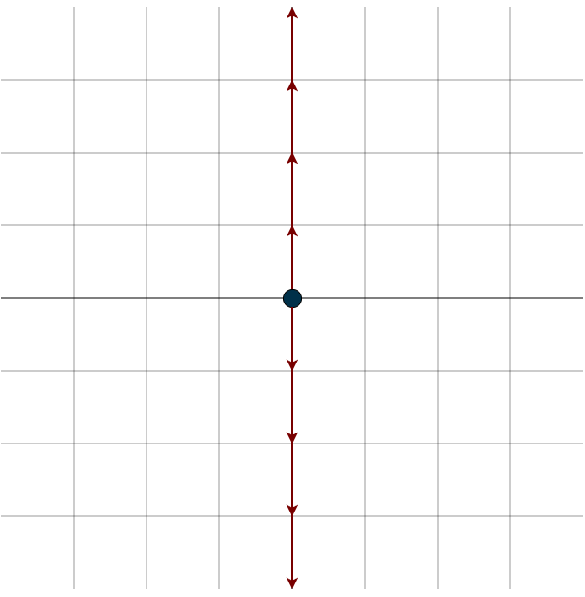
You can see that this whole line of vectors gets crushed down to the zero vector by this dimension crusher matrix. Remember, the subspaces of \(\mathbb{R}^n\) include \(\{0\}\), lines, planes, or hyperplanes through the origin. Depending on the matrix, the null space can be any of these subspaces. Geometrically, this means that every vector on that line, plane, or hyperplane is sent to zero after the transformation. It could even be the entire space, take, for example, the following matrix:

\(A = \begin{bmatrix} 0 & 0 \\ 0 & 0\end{bmatrix}\)

This one doesn’t discriminate; it sends every vector to zero. You might think of it like a black hole, sucking in everything around it. Also, the line of vectors that gets mapped to zero doesn’t have to align with the axes. For example, if you take \(A=\begin{bmatrix} 1 & 1 \end{bmatrix}\), the line representing its null space is diagonal, try calculating it yourself.

Finding the basis of the nullspace works the same way for any matrix size. (In short, you put the matrix into reduced row echelon form and identify the free variables).

Column Space / Range

I already mentioned what the range of a function is at the beginning of this chapter. The idea is the same for linear transformations. Basically, the range is the set of all vectors that the linear transformation can actually reach:

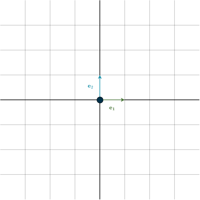
We can express the same idea using matrices (and personally, I prefer this viewpoint). The columns of a matrix are vectors, specifically, they’re the transformed basis vectors. When we multiply a matrix by a vector, we’re forming a linear combination of its columns. To refresh your memory, look at this matrix:

\(A = \begin{bmatrix} 1 & 2 \\ 5 & 7\end{bmatrix}\)

Multiplying it by a vector \(\mathbf{x}\) gives:

\(A\mathbf{x} = \begin{bmatrix} 1 & 2 \\ 5 & 7\end{bmatrix}\begin{bmatrix} x_1 \\ x_2\end{bmatrix} = \begin{bmatrix} 1 \\ 5 \end{bmatrix} \cdot x_1 + \begin{bmatrix} 2 \\ 7 \end{bmatrix} \cdot x_2\)

Remember: the span of a list of vectors is the set of all linear combinations of those vectors. In this case, the vectors are the columns of \(A\). Since these columns are linearly independent, their span is all of \(\mathbb{R}^2\). This span of the columns has a special name: the column space. It is dentoted as \(\text{Col}(A)\), for any given matrix \(A\). The name is fitting, it’s the vector space described by the columns of the matrix. The column space tells you exactly which vectors the matrix can produce. And importantly, it doesn’t always fill the whole space. Consider the matrix:

\(A = \begin{bmatrix} 1 & 2 \\ 1 & 2\end{bmatrix}\)

Here the columns are multiples of each other. This means the two different basis vectors are both mapped into the same one-dimensional span of the vector \((1,1)\).

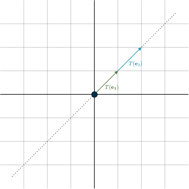
The black dotted line represents the column space of the matrix. Notice that it’s only one-dimensional and doesn’t cover the entire space. Similarly, in higher-dimensional spaces, the column space can be a line, plane, or hyperplane through the origin. It also doesn’t need to fill the entire space.

Since the column space is built from the transformed basis vectors, it should be no surprise that it sits inside \(\mathbb{R}^m\). It is a subspace of the output space. One more helpful fact: if a linear transformation is surjective, then every possible output vector can be produced. In that case, the range, i.e., the column space, is the entire output space.

Fundamental Theorem of Linear Transformations

The next definition is quite important as the name suggets:

So, once you know the dimension of the column space and the dimension of the input space as a whole, you can calculate the dimension of the null space. The reverse is also true: knowing the null space dimension allows you to find the dimension of the column space. This definition leads to two very useful tricks:

1. Checking whether a transformation has a non-trivial nullspace

Consider an \(m \times n\) matrix. If \(m<n\), the matrix is essentially downscaling: it maps a higher-dimensional space into a lower-dimensional one. The “lost’’ dimensions must go somewhere, they collapse to zero in the nullspace. Therefore, whenever \(m<n\), the linear transformation cannot be injective.

For example, if a transformation maps a 5-dimensional space into a 3-dimensional one, then 2 dimensions are lost in the process. Those 2 dimensions form the nullspace.

If \(m<n\), the matrix is wide, as you can clearly see:

\(\begin{bmatrix}x & x & x &x & x \\ x & x & x &x & x \end{bmatrix}\)

2. Checking at a glance whether the column space can fill the entire output space

Now consider the opposite situation. If \(m>n\), the matrix is “upscaling’’, trying to map a lower-dimensional space into a higher-dimensional one. The lower-dimensional input cannot possibly fill the entire higher-dimensional output space. This means the transformation cannot be surjective. The column space will not equal the output space.

For instance, mapping a 2-dimensional space into a 3-dimensional one produces a 2D plane sitting inside 3D space. No matter how you stretch, rotate, or skew it, that plane can never fill the entire 3D space, just like a sheet of paper cannot touch every point in your room. Vectors above or below the plane simply cannot be reached.

If \(m>n\), the matrix is tall, as you can clearly see:

\(\begin{bmatrix}x & x \\ x & x \\ x & x\\ x & x\\ x & x\end{bmatrix}\)

Summary

• Every linear transformation \(T\) comes with two subspaces: the nullspace and the column space.
• Every vector that \(T\) sends to zero ends up in the nullspace.
• Every vector that \(T\) can actually reach lies in the column space (range).
• These satisfy the relationship: \(\text{dim } V = \text{dim(null } T) + \text{dim(range } T)\).
• If \(m<n\) (a wide matrix), the nullspace will be larger than just \(\{0\}\).
• If \(m>n\) (a tall matrix), the column space will not span the whole output space.