Dot Product, Norms, and Vector Geometry
How can we measure the lengths, angles, and distances of vectors?
At the beginning of this course, we introduced the notion of a vector space: a set of objects called vectors that can be added and scaled by a scalar according to a few simple rules. Without adding any further structure, we explored how much can already be done with this definition alone. Using linear combinations, we generated new vectors from existing ones and saw how linear independence determines which sets are truly expressive. With the right set of vectors, every vector can be represented uniquely, a basis, and certain subsets of vectors can themselves form subspaces. We then studied linear transformations, which move vectors within the same space or into a different one, sometimes losing information in the process. We applied these concepts to real-world problems by solving linear systems, all without ever changing the underlying vector space itself. Now it is finally time to upgrade it. We will equip vector spaces with the ability to measure lengths of vectors and the angles between them, greatly expanding our problem-solving power.
Dot Product
For \(\mathbf{x}, \mathbf{y} \in \mathbb{R}^n\), the dot product of \(\mathbf{x}\) and \(\mathbf{y}\), denoted by \(\mathbf{x} \cdot \mathbf{y}\), is defined by
\(\mathbf{x} \cdot \mathbf{y} = x_1y_1 + \dots + x_ny_n\)
where \(\mathbf{x} = (x_1, \dots, x_n)\) and \(\mathbf{y} = (y_1, \dots, y_n)\).
Notice that the dot product takes two vectors as input and produces a single number as output, not another vector. This number tells us whether the vectors generally point in the same direction, and how strongly they are aligned. There are three possible cases:
1. Positive Dot Product
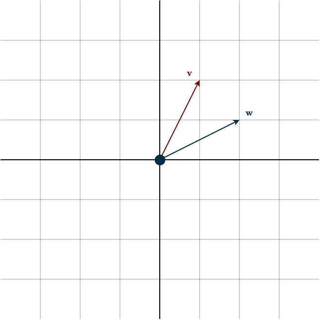
If the dot product of two vectors is positive, the vectors generally point in the same direction.
2. Negative Dot Product
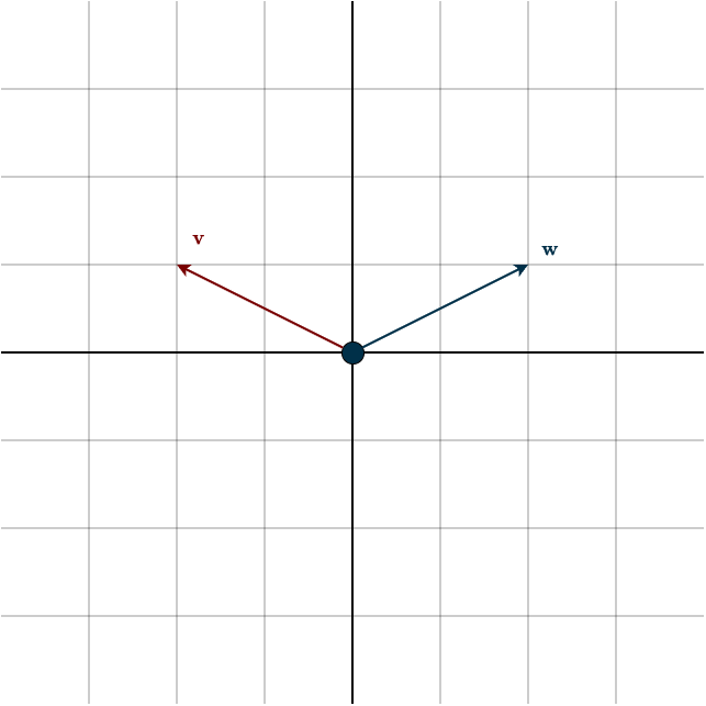
If the dot product is negative, the vectors generally point in opposite directions, or away from each other.
3. Dot Product equals zero (Important)
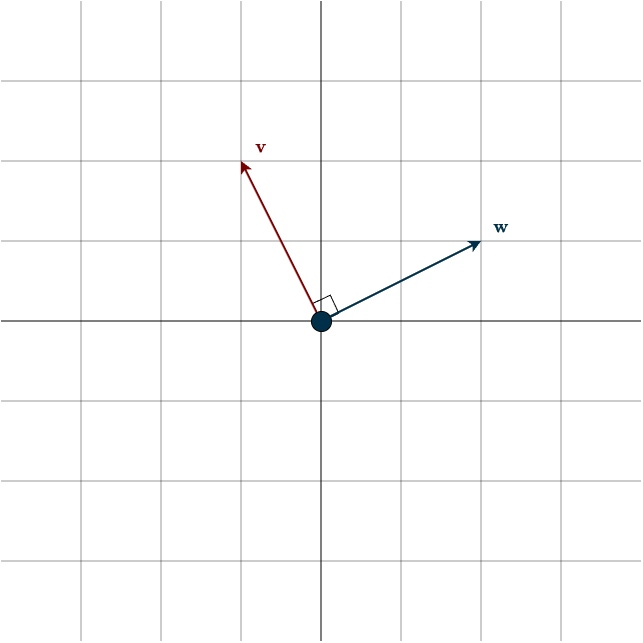
If the dot product is zero, the vectors are perpendicular to each other, that is, they meet at a 90° angle. This case is so important that it has a special name: orthogonal. Orthogonal vectors are simply vectors that are perpendicular to each other. (The term orthogonal is derived from the Greek word orthogonios, which translates to “right-angled.)
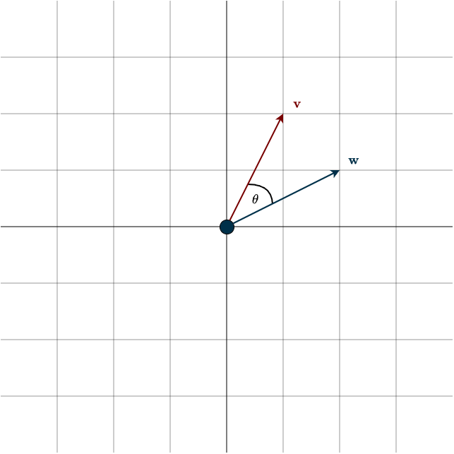
Imagine holding one vector fixed, let’s say \(\mathbf{w}\). Now consider an infinite line that passes through the origin and is perpendicular to \(\mathbf{w}\), like the span of the vector \(\mathbf{v}\) in the figure above. This line divides space into two halves. If the other vector in the dot product lies in the same half-space as \(\mathbf{w}\), the dot product will be positive. If it lies in the opposite half-space, the dot product will be negative. Finally, if it lies exactly on the perpendicular line that separates the two regions, the dot product will be zero.
An interesting fact is that the zero vector \(\mathbf{0}\) is orthogonal to every vector, since its dot product with any vector is zero. It is the only vector that is orthogonal to itself.
This last case really matters, since it sets the groundwork for everything that comes next. Before moving on, make sure you’re comfortable with it. A good way to build that intuition is to walk through a simple dot product example.
Example
Consider the following vectors:
\(\mathbf{v} = \begin{bmatrix} 7\\ 0 \\ 6 \end{bmatrix}, \hspace{1cm} \mathbf{w} = \begin{bmatrix} 1 \\ 9 \\ 8 \end{bmatrix}\)
Their dot product is:
\(\mathbf{v} \cdot \mathbf{w} = 7 \cdot 1 + 0 \cdot 9 + 6 \cdot 8 = 7 + 48 = 55\)
Because the result is positive, we know the two vectors are pointing roughly in the same direction. On its own, the number \(55\) might feel a bit random, it doesn’t immediately tell us how aligned the vectors really are. To get a more intuitive answer, we can go one step further and compute the exact angle between them. Look below for more info on that.
Some good to know properties about the dot product are the following:
- \(\mathbf{x} \cdot \mathbf{x} \geq 0\) for all \(\mathbf{x} \in \mathbb{R}^n\)
The dot product of a vector with itself is never negative. This makes sense if you think about vector length, lengths are always non-negative. In fact, this property is directly tied to how vector length is defined. We’ll come back to this shortly. - \(\mathbf{x} \cdot \mathbf{x} = 0\) if and only if \(\mathbf{x} = \mathbf{0}\).
If a vector has zero dot product with itself, then it must be the zero vector. - \(\mathbf{x} \cdot \mathbf{y} = \mathbf{y} \cdot \mathbf{x}\) for all \(\mathbf{x}, \mathbf{y} \in \mathbb{R}^n\).
The dot product is commutative, meaning order does not matter.
In machine learning, the terms dot product and inner product are often used interchangeably, but this can be misleading. An inner product extends the idea of the dot product to more general vector spaces. The dot product is just one specific inner product, and it’s the one we use in \(\mathbb{R}^n\). Inner products let us describe geometric ideas like lengths and angles even in spaces where the usual dot product doesn’t apply.
I won’t go into the full mathematical definition here, since it’s not our main focus. Just keep in mind that an inner product on \(V\) takes an ordered pair \((\mathbf{u},\mathbf{v})\) from \(V\) and returns a number \(\langle \mathbf{u}, \mathbf{v} \rangle \in F\), while following some rules.
Inner Product Space
An inner product space is simply a vector space equipped with an inner product. In our case, that inner product is the dot product. Here is the formal definition:
An inner product space is a vector space \(V\) along with an inner product on \(V\).
In this space, we can measure angles, lengths, and distances, something we could not do previously. Speaking of which, how do we actually measure the length of a vector?
Norms
The norm of a vector refers to its length, the distance from the origin to the tip of the arrow. To see where this comes from, let’s briefly recall the Pythagorean theorem. If you haven’t thought about it in a while, here’s the key idea. Take a right-angled triangle (see the figure). The length of the longest side, the hypotenuse, is given by
\(a^2 = b^2 + c^2\)
where \(a\) is the hypotenuse.
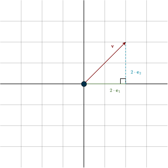
Now look at the vector \(\mathbf{v}\) in the figure. If we decompose it into its horizontal and vertical components, those components form the two perpendicular sides of a right triangle. The vector \(\mathbf{v}\) itself is the hypotenuse. So its length is exactly the quantity we get from the Pythagorean theorem.
At this point, one subtle but important choice enters the picture: the basis vectors define our coordinate system. We choose the standard basis vectors \(\mathbf{e}_1\) and \(\mathbf{e}_2\) to have length \(1\). This isn’t the result of a theorem, it’s a definition, a choice. We simply decide that one unit step along either axis corresponds to one unit of length. This choice makes geometry and algebra line up nicely. The standard basis is a particular type of basis, specifically, an orthonormal one. See below for more details.
It’s worth emphasizing that this choice is not forced. We could stretch the axes, or choose basis vectors that aren’t perpendicular. In those cases, the formula for length would still exist, but it would be more complicated (see orthonormal basis section below). The simplicity we’re about to see comes from the fact that the standard basis vectors are orthonormal.
We denote the length (or norm) of a vector \(\mathbf{v}\) by \(||\mathbf{v}||\). Using the Pythagorean theorem, we get
\(||\mathbf{v}||^2 = (v_1 \cdot ||\mathbf{e}_1||)^2 +(v_2 \cdot ||\mathbf{e}_2||)^2 = v_1^2 + v_2^2\)
since \(||\mathbf{e}_1|| = ||\mathbf{e}_2|| = 1\).
This expression should look familiar. In fact, it is exactly the dot product of a vector with itself:
\(||\mathbf{v}||^2 = \mathbf{v} \cdot \mathbf{v}\)
To get the actual length, we simply take the square root:
\(||\mathbf{v}|| = \sqrt{\mathbf{v} \cdot \mathbf{v}} = \sqrt{v_1^2 + v_2^2}\)
In our concrete example from the figure, where \(\mathbf{v}=(2,2)\), this gives
\(||\mathbf{v}|| = \sqrt{2^2 + 2^2} = \sqrt{8}\)
The mathematical definition is as follows:
For \(\mathbf{v} \in V\), the norm of \(\mathbf{v}\), denoted by \(||\mathbf{v}||\), is defined by
\(||\mathbf{v}|| = \sqrt{\langle \mathbf{v}, \mathbf{v} \rangle}\)
Note that \(\langle \mathbf{v}, \mathbf{v} \rangle\) denotes the inner product. This is the dot product in our specific vector space \(\mathbb{R}^n\). Some basic facts about norms worth remembering are:
- \(||\mathbf{v}|| = 0\) if and only if \(\mathbf{v} = \mathbf{0}\) with \(\mathbf{v} \in V\)
- \(||\lambda \mathbf{v}|| = |\lambda| ||\mathbf{v}||\) with \(\mathbf{v} \in V\) and for all \(\lambda \in F\)
Vectors with length \(1\) have a special name: unit vectors. For example, the standard basis vectors are all unit vectors. These vectors will play an important role later on. Any nonzero vector can be converted into a unit vector by dividing it by its length (norm). We call this process normalizing a vector:
$$\mathbf{u} = \frac{\mathbf{v}}{||\mathbf{v}||}$$
This is easy to understand intuitively. Think of the direction of a vector, along that same direction, there exists exactly one vector with length \(1\): the unit vector. Since the original vector points in the same direction, it must be a scaled version of that unit vector. The scaling factor is precisely the length of the vector. Dividing the vector by its length simply removes that scaling, shrinking (or expanding) the vector until its length becomes \(1\), while keeping its direction unchanged.
Angles Between Vectors
The dot product returns a number that tells us whether two vectors generally point in the same direction: positive if they do, negative if they do not. We also know that if the dot product is zero, then the vectors are perpendicular to each other, so there must be a connection to angles. The sign of the result immediately tells us whether the angle between the vectors is above 90° (dot product is negative) or below 90° (dot product is positive). (Remember the line analogy that splits space into two halves.)
When the two input vectors are unit vectors, something especially nice happens. Let’s call them \(\mathbf{u}_1\) and \(\mathbf{u}_2\). For now, just believe me with this result, we’ll explain where it comes from later in the chapter on projections.
\(\mathbf{u}_1 \cdot \mathbf{u}_2 = \cos(\theta)\)
Rearranging the equation gives
\(\theta = \cos^1(\mathbf{u}_1 \cdot \mathbf{u}_2)\)
This expression only works when both vectors have length \(1\). For general nonzero vectors \(\mathbf{v}_1\) and \(\mathbf{v}_2\), the fix is simple: normalize them by dividing each vector by its length.
$$\theta = \cos^{-1}(\frac{\mathbf{v}_1}{||\mathbf{v}_1||} \cdot \frac{\mathbf{v}_2}{||\mathbf{v}_2||}) = \cos^{-1}(\frac{\mathbf{v}_1 \cdot \mathbf{v}_2}{||\mathbf{v}_1||||\mathbf{v}_2||})$$
The expression inside the inverse cosine is what’s commonly called cosine similarity in machine learning. As the name suggests, it measures how similar two vectors are by looking at the angle between them, rather than their raw size. You might wonder why we don’t just use the dot product directly. The reason is that the dot product depends on vector length, while cosine similarity intentionally removes that effect. In many applications, vectors represent data where the direction carries meaning and the magnitude does not.
Finally, notice that once vectors are normalized, cosine similarity reduces to the dot product itself. For unit vectors, comparing angles and taking dot products end up being exactly the same thing. Let’s look at an example to make this more clear.
Example
Consider the following vectors:
\(\mathbf{v} = \begin{bmatrix} 1 \\ 2 \end{bmatrix}, \hspace{1cm} \mathbf{w} = \begin{bmatrix} 2 \\ 1 \end{bmatrix}\)
By plugging the numbers into the formula above, we get:
$$\theta = \cos^{-1}(\frac{1 \cdot 2 + 2 \cdot 1}{\sqrt{1 + 4} \cdot \sqrt{4 + 1}}) = \cos^{-1} \big( \frac{4}{5} \big) \approx 36.87°$$
Distance Between Vectors
A distance is simply a way of assigning a number to represent how far apart two points are. Geometrically, this is easy to visualize. Imagine two vectors in space, let’s focus on the tips of these arrows.

We want to measure the distance between them (dotted line in a figure). To do this, recall what vector subtraction looks like:

Notice something? The distance we’re looking for seems to be exactly the difference vector. But we want a number, not a vector. So a natural idea is to take the length of that difference vector, since its length literally measures how far apart the points are.
This is exactly the definition of Euclidean distance:
\(d(\mathbf{w}, \mathbf{v}) = ||\mathbf{w} \; – \; \mathbf{v}|| = \sqrt{\langle \mathbf{w} \; – \; \mathbf{v}, \mathbf{w} \; – \; \mathbf{v} \rangle} = \sqrt{(w_1 – v_1)^2 + (w_2 – v_2)^2}\)
You might remember that subtraction is not commutative, the order matters. But since we’re only looking at the length and not the direction, the order doesn’t matter here: both \(\mathbf{w} \; − \; \mathbf{v}\) and \(\mathbf{v} \; − \; \mathbf{w}\) have the same length.
This idea of distance will play an important role later when we develop real machine learning algorithms, like k-nearest neighbors. Since the Euclidean distance is only one way to measure how far apart two vectors are, I’ll briefly explain the distinction between a distance and a metric.
A metric is a well-behaved distance function that obeys certain mathematical rules, such as:
- Non-negativity: the distance can never be negative.
- Symmetry: \(d(\mathbf{v}, \mathbf{w})=d(\mathbf{w}, \mathbf{v})\).
- \(d(\mathbf{v}, \mathbf{w}) = 0 \hspace{0.25cm} \Leftrightarrow \hspace{0.25cm} \mathbf{v} = \mathbf{w}\)
Two points have zero distance between them exactly when they are the same point. - Triangle inequality: \(d(\mathbf{v}, \mathbf{w}) \leq d(\mathbf{v}, \mathbf{u}) + d(\mathbf{u}, \mathbf{w})\) (see section below for more info)
A distance, on the other hand, is just any way of assigning a number to “how far apart” two points are. Every metric is a distance, but not every distance is a metric, some distance-like functions may fail the triangle inequality, or might assign zero to points that aren’t equal (which would be confusing, since distance should indicate separation).
A metric is a generalization of the Euclidean distance we are used to. However, depending on the problem, different metrics might be better suited. For example, besides Euclidean distance, we also have Manhattan distance, cosine distance, and others. Finally, be careful not to confuse the term metric here (meaning a distance function following some rules) with the other use of the word metric in machine learning, which refers to performance evaluation of models.
A Note on the Cauchy–Schwarz and Triangle Inequalities
When we move from 2D or 3D space to high-dimensional vectors, we want familiar geometric ideas to continue making sense: length, angle, distance, and projection. But these concepts do not automatically behave well just because we define an inner product. What makes this geometry actually work are two fundamental inequalities. They quietly enforce the structure that allows inner product spaces to behave like the Euclidean space we are used to.
1. Cauchy Schwarz :
\(| \mathbf{u} \cdot \mathbf{v}| \leq ||\mathbf{u}|| ||\mathbf{v}||\)
This inequality guarantees that the cosine similarity formula always produces values in the interval \([−1,1]\). That fact is essential, because cosine, and therefore the inverse cosine, is only defined on this interval. There is no angle whose cosine is \(1.3\) or \(−2\). Such numbers simply do not correspond to any rotation in space. So if we want the phrase “angle between two vectors” to mean anything real, the quantity we pass into \(\cos^{−1}\) must lie between \(−1\) and \(1\).
To see why this matters, consider the dot product by itself:
\(\mathbf{u} \cdot \mathbf{v}\)
There is no built-in limit on how large or small this value can be. By scaling the vectors, we can make the dot product arbitrarily large in magnitude. Cauchy–Schwarz is what prevents this from breaking our geometry:
\(| \mathbf{u} \cdot \mathbf{v}| \leq ||\mathbf{u}|| ||\mathbf{v}||\)
Dividing both sides by \(||\mathbf{u}||||\mathbf{v}||\):
$$ \left| \frac{\mathbf{u} \cdot \mathbf{v}}{||\mathbf{u}|| ||\mathbf{v}||} \right| \leq 1 $$
Because of the absolute value, this immediately tells us that the result must lie in \([−1,1]\). This is the precise reason angles and cosine similarity are well-defined in inner product spaces.
2. Triangle Inequality
\(||\mathbf{u} + \mathbf{v}|| \leq ||\mathbf{u}|| + ||\mathbf{v}||\)
The triangle inequality guarantees that the direct path is always the shortest path. In other words, taking a detour can never be cheaper than going straight. This is what makes norms behave like real distances. Without this property, distances could be “cheated”: a longer, indirect path could end up shorter than a direct one. At that point, the concept of distance would lose its meaning entirely. Distance plays a central role in machine learning: gradient-based optimization, nearest-neighbor methods, clustering, and embedding spaces all rely on it behaving sensibly. The triangle inequality is what ensures that this assumption holds.
Simply said: Cauchy–Schwarz controls angles. The triangle inequality controls distance. Together, they are the reason inner product spaces feel familiar, even in thousands of dimensions. They form the mathematical backbone that allows geometric intuition to survive in machine learning. You don’t need to know their proofs to use them effectively. What matters is understanding that these two powerful inequalities are always working quietly in the background, making everything else possible.
Orthonormal Basis
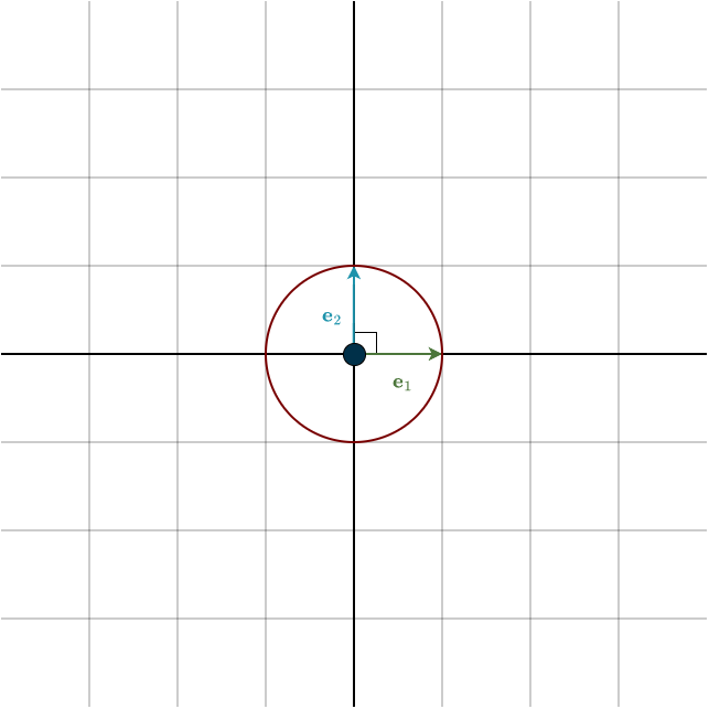
I want to briefly highlight what an orthonormal basis is, since it will be important later on. Recall that we need a basis to create coordinate representations and, in turn, matrices. However, the choice of basis is completely up to us, and there are many options. Among them is a special class called an orthonormal basis. “Ortho” means orthogonal, and “normal” means unit length, that is, length one. Simply put, in such a basis every vector is perpendicular to every other vector, and all of them have length \(1\). The standard basis is a perfect example of this, but there are others, namely, rotated versions of it. In \(\mathbb{R}^2\), these form the unit circle, a circle of radius one, and in \(\mathbb{R}^3\), the unit sphere.
This special choice of basis greatly simplifies computations, because all cross terms vanish. Earlier, when defining the length of a vector, I mentioned that things simplify because we are using an orthonormal basis. Here is why. Suppose we want to compute the squared length of a vector \(\mathbf{v}\). Written in terms of the basis vectors \(\mathbf{e}_1\) and \(\mathbf{e}_2\), we have
\(\mathbf{v} = v_1 \cdot \mathbf{e}_1 + v_2 \cdot \mathbf{e}_2\)
By definition, the squared length of \(\mathbf{v}\) is
\(||\mathbf{v}||^2 = \mathbf{v} \cdot \mathbf{v}\)
Substituting the expression for \(\mathbf{v}\), we obtain
\( \begin{align*}||\mathbf{v}||^2 &= \mathbf{v} \cdot \mathbf{v} \\\\
&= (v_1\mathbf{e}_1 + v_2\mathbf{e}_2) \cdot (v_1\mathbf{e}_1 + v_2\mathbf{e}_2) \\\\
&= v_1^2 (\mathbf{e}_1 \cdot \mathbf{e}_1) + v_1 v_2 (\mathbf{e}_1 \cdot \mathbf{e}_2) + v_2 v_1 (\mathbf{e}_2 \cdot \mathbf{e}_1) + v_2^2( \mathbf{e}_2 \cdot \mathbf{e}_2) \end{align*}\)
Because the basis is orthonormal, we have
\(\mathbf{e}_1 \cdot \mathbf{e}_2 = 0 \hspace{0.5cm}\) and \(\hspace{0.5cm} \mathbf{e}_1 \cdot \mathbf{e}_1 = \mathbf{e}_2 \cdot \mathbf{e}_2 = 1\)
Applying these facts gives
\( \begin{align*} ||\mathbf{v}||^2 &= v_1^2 \cdot 1 + v_2^2 \cdot 1 + 2 v_1 v_2 \cdot 0 \\\\ &= v_1^2 + v_2^2\end{align*}\)
This is what is meant by cross terms canceling out: whenever two different basis vectors appear in a dot product, the result is zero because they are orthogonal. On the other hand, dotting a basis vector with itself gives one, since each basis vector has unit length. As a result, the squared length reduces to a simple sum of squares of the coordinates. If we do not have an orthonormal basis, these cross terms do not disappear and the coordinates are scaled, which makes the calculation slightly more annoying.
Summary
- By equipping a vector space with an inner product, we gain the ability to measure lengths, angles, and distances.
- In the special case of \(\mathbb{R}^n\), the inner product is the dot product: \(\mathbf{u} \cdot \mathbf{v}\). It tells us whether two vectors generally point in the same direction. If the result is positive, they point in the same direction; if it is negative, they point in opposite directions.
- There is a special case where the dot product is zero. In this case, the vectors are called orthogonal, meaning they are perpendicular to each other.
- The length, or norm, of a vector is defined using the inner product: \(||\mathbf{v}|| = \sqrt{\langle \mathbf{v}, \mathbf{v} \rangle}\). Vectors with length one are called unit vectors. Normalizing a vector means turning any nonzero vector into a unit vector.
- The dot product also allows us to measure the exact angle between two vectors: \(\theta = \cos^{-1}(\frac{\mathbf{v}_1 \cdot \mathbf{v}_2}{||\mathbf{v}_1||||\mathbf{v}_2||})\)
- The distance between two vectors is simply the length of their difference vector.
- Two inequalities ensure that this geometry works the way we are used to: Cauchy–Schwarz, which controls angles, and the triangle inequality, which controls distances.
- A basis is called orthonormal when each vector has length one and is perpendicular to all the others. It simplifies calculations.