Matrices
How can we represent linear transformations numerically?
We have seen the power that a linear transformation can wield, but now we need a way to harness it. To do this, we require a numerical representation that allows computers to perform the work for us. We call these representations matrices. Matrices capture much of the information we explored in the previous chapter through their structure and the rules that govern their interactions. But take note: matrices do not only represent linear transformations, they can also represent vectors and more. Context is everything.
Linear Transformations in Numbers
In the last chapter, we talked about a machine that moves vectors, what we called a linear transformation. Recall that to describe such a transformation completely, it’s enough to know where it sends the basis vectors:
\(T(\mathbf{v}_1), T(\mathbf{v}_2), \dots, T(\mathbf{v}_n)\) for an input basis \(\mathcal{B} = (\mathbf{v}_1, \mathbf{v}_2, \dots, \mathbf{v}_n)\)
Now we might ask: Is there a way to represent this transformation numerically, in a compact and organized form?
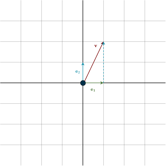
Let’s consider a simple case. Suppose both our input and output spaces are \(\mathbb{R}^2\), and both use the standard basis. Our linear transformation will be a leftward shear. The standard basis vectors are
\(\mathbf{e}_1 = \begin{bmatrix} 1\\ 0\\ \end{bmatrix}, \hspace{1cm} \mathbf{e}_2 = \begin{bmatrix} 0\\ 1\\ \end{bmatrix}\)
After applying the transformation, these basis vectors become
\(T(\mathbf{e}_1) = \begin{bmatrix} 1\\ 0\\ \end{bmatrix}, \hspace{1cm} T(\mathbf{e}_2) = \begin{bmatrix} -1\\ 1\\ \end{bmatrix}\)
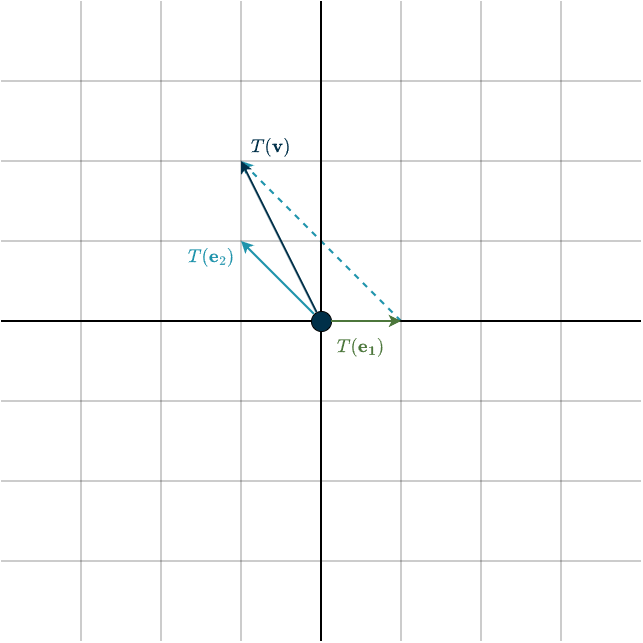
Since every output vector is a linear combination of \(T(\mathbf{e}_1)\) and \(T(\mathbf{e}_2)\), these two transformed basis vectors contain all the information we need for a compact representation of the transformation. So let’s simply place them next to each other:
\(T(\mathbf{e}_1), T(\mathbf{e}_2)= \begin{bmatrix} 1\\ 0\\ \end{bmatrix}, \begin{bmatrix} -1\\ 1\\ \end{bmatrix}\)
This notation is a bit awkward. To clean it up, we drop the middle bracket and arrange them neatly like this:
\(A = \begin{bmatrix} T(\mathbf{e}_1) & T(\mathbf{e}_2) \end{bmatrix} = \begin{bmatrix} 1 & -1\\ 0 & 1\\ \end{bmatrix}\)
This, ladies and gentlemen, is what we call a matrix. It’s a rectangular array of numbers that encodes a linear transformation.
We denote matrices by capital letters, and the standard choice is the letter \(A\). Now you might wonder: for an arbitrary input vector, how do we calculate where it ends up under this transformation? Think of \(A\) as a machine that moves vectors. You feed \(A\) any input vector, and it returns the transformed vector according to the linear transformation it represents. We compute this using matrix–vector multiplication:
\(A\mathbf{v} = \begin{bmatrix} 1 & -1\\ 0 & 1\\ \end{bmatrix}\begin{bmatrix} v_1\\ v_2\\ \end{bmatrix} = \begin{bmatrix} 1\\ 0\\ \end{bmatrix} \cdot v_1 + \begin{bmatrix} -1\\ 1\\ \end{bmatrix} \cdot v_2 = T(\mathbf{e}_1) \cdot v_1 + T(\mathbf{e}_2) \cdot v_2\)
Multiplying a matrix by a vector produces exactly the linear combination of the transformed basis vectors that we discussed in the previous chapter. (Matrix–vector multiplication is defined this way on purpose so that everything stays consistent.) Notice what happens: the coordinates of the input vector \(\mathbf{v}\) no longer scale the original basis vectors, they now scale the transformed basis vectors. By the linearity of our transformation, this guarantees that the resulting combination is precisely the correct transformed vector. In summary: the matrix is built to send the basis vectors to their correct places, and linearity ensures that every other vector is transformed correctly as well.
To create a matrix representation of a linear transformation in general, the first step is to choose a basis for each of the vector spaces involved. A matrix only exists relative to a choice of basis, no basis means no matrix. Once a basis is chosen, the resulting matrix representation is unique for that basis. Recall that the same linear transformation can look different under different bases: the transformation itself doesn’t change, but its matrix does.
After choosing bases, the next step is to transform the input basis vectors, producing the familiar list \(T(\mathbf{v}_1), T(\mathbf{v}_2), \dots, T(\mathbf{v}_n)\). If the transformed vectors are not already expressed in the output basis, we must rewrite them in that basis. This step is crucial; otherwise, the resulting matrix will be incorrect. For each input basis vector \(\mathbf{v}_k\), there exists a linear combination of the output basis vectors such that
\(T(\mathbf{v}_k) = a_1 \cdot \mathbf{w}_1 + a_2 \cdot \mathbf{w}_2 + \dots + a_m \cdot \mathbf{w}_m\)
The scalars \(a_1, \dots, a_m\) become the entries of the matrix. For example, suppose the transformation of the first basis vector \(\mathbf{v}_1\) can be expressed (arbitrarily chosen for illustration) as
\(T(\mathbf{v}_1) = 2 \cdot \mathbf{w}_1 + 3 \cdot \mathbf{w}_2\)
The numbers \(2\) and \(3\) are then placed into the first column of the matrix \(A\). A column is a vertical slice of a matrix, running from top to bottom, as shown in red below:
\(\begin{bmatrix} \color{red}{2} & ? \\ \color{red}{3} & ?\\ \end{bmatrix}\)
The question-mark slot is then filled with the coordinates of the second transformed basis vector, expressed in the output basis. This becomes the second column of the matrix. You repeat this process for all remaining basis vectors, and once each column is filled, your matrix is complete.
Next, we will take a closer look at the structure of the matrix.
Structure of a Matrix
Earlier, we saw what a column of a matrix is. A row is similar, but instead of running vertically, it is a horizontal slice of the matrix. The figure below illustrates both rows and columns:
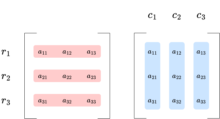
The letter \(r\) stands for rows and \(c\) stands for columns. We navigate a matrix using indices, the small numbers written below the entries. These indices tell us which row and column a given scalar occupies. The first index refers to the row, and the second to the column. For example, \(a_{23}\) is the entry in the second row and third column.
Remember that a matrix is simply a representation of a linear transformation with respect to a chosen basis, and this meaning is reflected directly in the matrix’s structure. Each column corresponds to one transformed basis vector from the input space, as we saw above. Therefore, if the input vector space is \(\mathbb{R}^n\), we have \(\text{dim}(\mathbb{R}^n) = n\), which means \(n\) basis vectors, thus the matrix has \(n\) columns.
These transformed basis vectors live in the output space \(\mathbb{R}^m\), and their coordinates specify how to scale each output basis vector. Since \(\text{dim}(\mathbb{R}^m) = m\), there are \(m\) coordinates, and therefore \(m\) rows in the matrix. Altogether, this gives us an \(m \times n\) matrix.
For example, a \(3 \times 3\) matrix represents a linear transformation from \(\mathbb{R}^3\) to \(\mathbb{R}^3\), a transformation from a space to itself. A \(5 \times 3\) matrix corresponds to a transformation from \(\mathbb{R}^3\) to \(\mathbb{R}^5\). (Pay close attention to the order: it is an \(m \times n\) matrix, but the map is \(T:\mathbb{R}^n \rightarrow \mathbb{R}^m\).)
In general, if \(T\) is a linear transformation from an \(n\)-dimensional vector space to an \(m\)-dimensional one, then its matrix representation is \(m \times n\). The special case where \(m = n\) gives a square matrix, which corresponds to a transformation from a vector space to itself. Most matrices, however, are rectangular.

In nearly all textbooks and university exercises, the standard basis is used unless stated otherwise. Now, how exactly do we multiply matrices?
Matrix Multiplication
Matrices represent linear transformations, so multiplying matrices is simply composing those transformations. Recall that the product / composition of linear transformations must be well defined, meaning the vector spaces have to match. If you have \(S: U \rightarrow V\) and \(T: V \rightarrow W\), the composition \(T \circ S\) is well defined because the codomain of \(S\) matches the domain of \(T\) (the output of \(S\) is in \(V\), and the input of \(T\) is in \(V\)). This same condition appears in matrix multiplication. The shapes must align: the number of columns of the first matrix must equal the number of rows of the second. So if you have an \(m \times n\) matrix, it can only multiply a matrix of the form \(n \times h\). For example, a \(3 \times 5\) matrix multiplied by a \(3 \times 7\) matrix is not defined.
Determining the shape of the product is easy. If an \(m \times n\) matrix is multiplied by an \(n \times h\) matrix, the result will have shape \(m \times h\). The middle dimension cancels out, much like skipping the intermediate space when composing transformations.
Also remember that the composition of linear transformations is not commutative. Thus, for two matrices \(A\) and \(B\), we generally have
\(AB \neq BA\)
Each matrix moves vectors. Multiplying two matrices means performing one movement followed by the other in sequence. The resulting product matrix represents this combined transformation as a single, smooth, unified movement.
Note that we read matrix multiplication from right to left, just like the composition of linear transformations. In the product \(AB\), \(B\) is applied first, followed by \(A\).
There are different ways to compute the matrix product \(AB\) numerically:
1. Row of A times column of B:
You take what is called the dot product between each row of \(A\) and each column of \(B\). We will define the dot product more formally later, but for now you only need to know how to compute it:
\(c_{11}= a_{11} \cdot b_{11} + a_{12} \cdot b_{21} + a_{13} \cdot b_{31} \)
So for the given matrices:
\(A = \begin{bmatrix} 1 & 2 & 3\\ 4 & 5 & 6\\ 7 & 8 & 9 \end{bmatrix}, \hspace{1cm} B = \begin{bmatrix} 1 & 2 & 5\\ 7 & 6 & 2\\ 4 & 3 & 2\end{bmatrix}\)
The upper left entry of \(AB\) would be:
\(AB_{11} = 1 \cdot 1 + 2 \cdot 7 + 3 \cdot 4= 27\)
You repeat this process for all remaining rows and columns.
2. Matrix A times every column of B:
Each column of \(AB\) is a linear combination of the columns of \(A\). Another way to see this is to perform matrix–vector multiplication with \(A\) on every column vector of \(B\) (columns of \(B\) are denoted by \(b_{\mathrm{\,I}}, b_{\mathrm{\,II}} \dots b_p\)):
\(AB = \begin{bmatrix} A b_{\mathrm{\,I}}, A b_{\mathrm{\,II}} \dots A b_p \end{bmatrix}\)
Using the same matrices as above, the first column of \(AB\) is:
\(AB_{*1} = Ab_{\mathrm{\,I}} = \begin{bmatrix} 1 & 2 & 3\\ 4 & 5 & 6\\ 7 & 8 & 9 \end{bmatrix} \begin{bmatrix} 1\\ 7\\ 4\end{bmatrix} = \begin{bmatrix} 1\\ 4\\ 7\end{bmatrix} \cdot 1 + \begin{bmatrix} 2\\ 5\\ 8\end{bmatrix} \cdot 7 + \begin{bmatrix} 3\\ 6\\ 9\end{bmatrix} \cdot 4 = \begin{bmatrix} 27\\ 63\\ 99\end{bmatrix}\)
Repeat this process for each remaining column of \(B\).
The matrix \(B\) first moves the standard basis vectors to new positions according to the transformation it represents. These transformed basis vectors form the columns of \(B\). Then \(A\) takes these already-transformed basis vectors and moves them again to the positions described by the transformation of \(A\). This is what multiplying the columns of \(B\) with the matrix \(A\) shows.
3. Every row of A times matrix B:
Every row of \(AB\) is a combination of the rows of \(B\). This is similar to the previous approach, except now we work with rows instead of columns. Specifically, each row of \(A\) multiplies the matrix \(B\):
\(\begin{bmatrix} \text{row } i \text{ of } A \end{bmatrix}B = \begin{bmatrix} \text{row } i \text{ of } AB \end{bmatrix}\)
Using the same matrices as above, the first row of \(AB\) is:
\(AB_{1*} = \begin{bmatrix} 1 & 2 & 3 \end{bmatrix} \begin{bmatrix} 1 & 2 & 5\\ 7 & 6 & 2\\ 4 & 3 & 2\end{bmatrix} = 1 \cdot \begin{bmatrix} 1 & 2 & 5 \end{bmatrix} + 2 \cdot \begin{bmatrix} 7 & 6 & 2\end{bmatrix} + 3 \cdot \begin{bmatrix} 4 & 3 & 2 \end{bmatrix} = \begin{bmatrix} 27 & 23 & 15 \end{bmatrix} \)
Apply the same process to all other rows of \(A\).
Essentially, you can view the same matrix multiplication from two angles: left multiplication and right multiplication. If we have \(AB\), we can think of it as multiplying \(B\) on the left with \(A\), which means that \(A\) transforms the rows of \(B\). But we can also see it as \(B\) multiplying \(A\) on the right, which tells us that \(B\) transforms the columns of \(A\). Simply put: multiplying on the left transforms rows; multiplying on the right transforms columns.
A row vector is written horizontally, a column vector vertically. The orientation matters because column vectors are multiplied on the left by matrices, while row vectors multiply on the right. There is also a deeper mathematical reason for this, which we will explore in the chapter on transposes.
4. Columns Multiply Rows:
Here comes my favourite way of multiplying matrices: multiply columns \(1\) to \(n\) of \(A\) with rows \(1\) to \(n\) of \(B\), and then add the resulting matrices together:
\(AB = \begin{bmatrix} a_{11} & a_{12} & a_{13} \\ a_{21} & a_{22} & a_{23} \\ a_{31} & a_{32} & a_{33} \end{bmatrix} \begin{bmatrix} b_{11} & b_{12} & b_{13} \\ b_{21} & b_{22} & b_{23} \\ b_{31} & b_{32} & b_{33} \end{bmatrix} = \begin{bmatrix} a_{11} \\ a_{21} \\ a_{31} \end{bmatrix} \begin{bmatrix} b_{11} & b_{12} & b_{13}\end{bmatrix} + \begin{bmatrix} a_{12} \\ a_{22} \\ a_{32} \end{bmatrix} \begin{bmatrix} b_{21} & b_{22} & b_{23}\end{bmatrix} + \begin{bmatrix} a_{13} \\ a_{23} \\ a_{33} \end{bmatrix} \begin{bmatrix} b_{31} & b_{32} & b_{33}\end{bmatrix}\)
Basically, you take the first column of \(A\) and multiply it by the first row of \(B\), then do the same with the second column of \(A\) and the second row of \(B\), and so on. Adding all of these sub-results together gives you the final product. These sub-multiplications are known as outer products, which we will explore in more detail later. For now, just note that each scalar \(b_{ij}\) in a row of \(B\) scales the corresponding column vector of \(A\). While the dot product produces a single number, the outer product produces an entire matrix.
\(\begin{bmatrix} a_{11} \\ a_{21} \\ a_{31} \end{bmatrix} \begin{bmatrix} \color{red}{b_{11}} & \color{green}{b_{12}} & \color{orange}{b_{13}}\end{bmatrix} = \begin{bmatrix} a_{11} \cdot \color{red}{b_{11}} & a_{11} \cdot \color{green}{b_{12}} & a_{11} \cdot \color{orange}{b_{13}} \\ a_{21} \cdot \color{red}{b_{11}} & a_{21} \cdot \color{green}{b_{12}} & a_{21} \cdot \color{orange}{b_{13}} \\ a_{31} \cdot \color{red}{b_{11}} & a_{31} \cdot \color{green}{b_{12}} & a_{31} \cdot \color{orange}{b_{13}}\end{bmatrix}\)
You can just as well think of it the other way around: scaling the same row vector of \(B\) by the scalars in the column vector of \(A\). It gives the same result. I like this method of multiplying matrices because, for me, it is less error-prone, even if it takes a bit longer to write down all the intermediate matrices.
(Here’s a small, oversimplified tip in advance: column times row gives an outer product, whereas row times column gives a dot product. Just check the shapes. \(1 \times n\) multiplied with \(n \times 1\) will give you a number. \(n \times 1 \) mulitplied with \(1 \times n\) will give you a matrix. This way, you won’t mix them up right away. A little analogy that helps me is this: the inner product (that’s just the dot product in our case) is like a black hole, sucking all the numbers in and producing just a single scalar. The outer product is like an explosion, sending everything outward and creating a whole matrix.)
Using the same matrices again, we obtain the following:
\( \begin{align*}AB &= \begin{bmatrix} 1 \\ 4 \\ 7 \end{bmatrix} \begin{bmatrix} 1 & 2 & 5\end{bmatrix} + \begin{bmatrix} 2 \\ 5 \\ 8 \end{bmatrix} \begin{bmatrix} 7 & 6 & 2\end{bmatrix} + \begin{bmatrix} 3 \\ 6 \\ 9 \end{bmatrix} \begin{bmatrix} 4 & 3 & 2\end{bmatrix} \\\\ &= \begin{bmatrix} 1 & 2 & 5 \\ 4 & 8 & 20 \\ 7& 14 & 35\end{bmatrix} + \begin{bmatrix} 14 & 12 & 4 \\ 35 & 30 & 10 \\ 56 & 48 & 16\end{bmatrix} + \begin{bmatrix} 12 & 9 & 6 \\ 24 & 18 & 12 \\ 36 & 27 & 18\end{bmatrix} \\\\ &= \begin{bmatrix} 27 & 23 & 15 \\ 63 & 56 & 42 \\ 99 & 89 & 69\end{bmatrix}\end{align*}\)
I find it quite fascinating how the same numbers appear in different ways across these methods. All of these approaches to matrix multiplication produce the same result, so you can generally use whichever one feels most natural to you. However, there are situations where one method is definitely faster than the others. For example, when multiplying with a permutation matrix (we will see what that is shortly), the second or third method is usually the most efficient, depending on whether the permutation matrix is on the left or the right of \(A\).
Remark: Imagine you have a matrix \(A\) and you want to multiply it by \(B\). Since \(AB \neq BA\), you must be explicit about which side you are multiplying \(A\) on. This distinction will play an important role later when we solve equations using matrices.
One more thing: you can take powers of matrices. In this sense, matrices behave like numbers:
\(A^p = AAA \dots A \;(\text{p times}), \hspace{1cm} (A^p)(A^q) = A^{p+q}, \hspace{1cm} (A^p)^q = A^{pq}\)
However, the matrix must be square for these expressions to make sense; otherwise, the multiplication would not be well defined. Note that \(p\) and \(q\) can be zero or negative; these rules still hold in those cases. We define \(A^0 = I\) (look at the section below for the meaning of \(I\)). This mirrors the familiar rule that any number raised to the power of \(0\) equals \(1\). For example \(2^0 = 1\).
Negative powers also work, but they are a bit more tricky. For numbers, \(a^{-1} = \frac{1}{a}\). For matrices, the analogue is \(A^{-1}\). However, the inverse of a matrix does not always exist, and we will examine this interesting topic shortly.
Finally, in the last chapter we saw that the product of linear transformations is associative and distributive, so you can already guess that matrix multiplication behaves the same way.
Identity Matrix
The identity matrix plays a fundamental role in linear algebra, so it’s worth highlighting explicitly. An identity, or neutral element, is one that leaves other elements unchanged under a given operation. In our context, the identity matrix is the matrix that does not alter any other matrix when used in matrix multiplication. We denote it by the special letter \(I\); it represents the identity linear transformation. In simple terms, it is the “do-nothing” matrix:
\(IA = AI = A\)
This is reflected clearly in its structure. In the \(2 \times 2\) case:
\(I_2 = \begin{bmatrix} 1 & 0 \\ 0 & 1 \end{bmatrix}\)
In the \(3 \times 3\) case:
\(I_3 = \begin{bmatrix} 1 & 0 & 0 \\ 0 & 1 & 0 \\0 & 0 & 1\end{bmatrix}\)
And in general:
\(I_n = \begin{bmatrix}
1 & 0 & \cdots & 0 \\
0 & 1 & \cdots & 0 \\
\vdots & \vdots & \ddots & \vdots \\
0 & 0 & \cdots & 1
\end{bmatrix}\)
The identity matrix does not move vectors, which is why its columns are exactly the unchanged basis vectors. Note that the identity matrix must be square, meaning it maps a vector space back to itself. If it were not square, it would take vectors into a different vector space, which would change them, contradicting the very definition of an identity transformation.
Matrix Addition
The sum of two matrices of the same size is the matrix obtained by adding corresponding entries in the matrices:
\(A + B = \begin{bmatrix} a_{11} & a_{12} & a_{13} \\ a_{21} & a_{22} & a_{23} \\ a_{31} & a_{32} & a_{33} \end{bmatrix} + \begin{bmatrix} b_{11} & b_{12} & b_{13} \\ b_{21} & b_{22} & b_{23} \\ b_{31} & b_{32} & b_{33} \end{bmatrix} = \begin{bmatrix} a_{11} + b_{11} & a_{12} + b_{12} & a_{13} + b_{13}\\ a_{21} + b_{21} & a_{22} + b_{22} & a_{23} + b_{23}\\ a_{31} + b_{31} & a_{32} + b_{32} & a_{33} + b_{33} \end{bmatrix}\)
Same size doesn’t necessarily mean square matrices; the matrices could also be rectangular, as long as their shapes match. For example, given the matrices:
\(A = \begin{bmatrix} 1 & 2 \\ 2 & 4 \\ 7 & 3 \end{bmatrix}, \hspace{1cm} B = \begin{bmatrix} 7 & 2 \\ 5 & 1 \\ 4 & 9 \end{bmatrix}\)
their sum is:
\(A + B = \begin{bmatrix} 1 + 7 & 2 + 2 \\ 2 + 5 & 4 + 1 \\ 7 + 4 & 3 + 9 \end{bmatrix} = \begin{bmatrix} 8 & 4 \\ 7 & 5 \\ 11 & 12 \end{bmatrix}\)
Note that matrix addition is commutative; it’s only matrix multiplication that isn’t.
Scalar Multiplication of a Matrix
The product of a scalar and a matrix is the matrix obtained by multiplying each entry in the matrix by the scalar:
\(\lambda \cdot A = \lambda \cdot \begin{bmatrix} a_{11} & a_{12} & a_{13} \\ a_{21} & a_{22} & a_{23} \\ a_{31} & a_{32} & a_{33} \end{bmatrix} = \begin{bmatrix} \lambda \cdot a_{11} & \lambda \cdot a_{12} & \lambda \cdot a_{13} \\ \lambda \cdot a_{21} & \lambda \cdot a_{22} & \lambda \cdot a_{23} \\ \lambda \cdot a_{31} & \lambda \cdot a_{32} & \lambda \cdot a_{33} \end{bmatrix}\)
For example:
\(5 \cdot A = 5 \cdot \begin{bmatrix} 1 & 2 \\ 3 & 4 \end{bmatrix} = \begin{bmatrix} 5 \cdot 1 & 5 \cdot 2 \\ 5 \cdot 3 & 5 \cdot 4 \end{bmatrix} = \begin{bmatrix} 5 & 10 \\ 15 & 20 \end{bmatrix}\)
(So the set of matrices is closed under addition as well as scalar multiplication. This should sound familiar, since these are the basic building blocks of a vector space. Those of you with a keen eye may have already noticed that matrices themselves form a vector space, but while that’s a neat observation, it won’t be our focus here.)
Vectors vs Matrices
You may wonder: what is the difference between a column vector and a matrix? After all, matrices can have any shape, which means a matrix could also be \(m \times 1\), the same shape as a column vector. For example, consider this box of numbers:
\(\begin{bmatrix} 1 \\ 4 \\ 8 \end{bmatrix}\)
Is it a vector or a matrix? Can a vector be a matrix? The answer is: you cannot tell without context. The same array of numbers could represent a vector or a linear transformation.
Mathematically, vectors are abstract objects in a vector space: they can be scaled, added, and moved by linear transformations. Think about geometric vectors. Vectors are not linear transformations themselves; they are the things being moved. Linear transformations, on the other hand, are functions that take vectors as input and output other vectors.
We represent vectors and linear transformations using matrices and coordinate systems so we can work with them efficiently. This creates a useful but sometimes confusing situation: the same array of numbers might represent a vector or a linear transformation. Thus, it is crucial to understand that a vector exists independently of any coordinates, while its matrix is merely the representation of that vector relative to a particular basis.
Later on, we will see the deeper mathematical reason why linear transformations can appear like vectors, even in their coordinate representation.
In applications, especially in coding and machine learning, context is key to understanding what a matrix actually represents.
Summary
- Matrices are coordinate representations of linear transformations.
- Given a basis, we create matrices by putting the transformed basis vectors in the columns.
- Matrix multiplication corresponds to the composition of linear transformations. It is not commutative, and and the shapes need to match.
- There are different ways to numerically calculate the product of two matrices; choose the method that best suits your needs.
- The identity matrix acts as a “do nothing” transformation, it leaves vectors unchanged.
- Always consider the context: the same array of numbers can represent a vector, a matrix, or another object, so pay attention to what the representation means.