Solving Systems of Linear Equations
How can we use what we’ve learned so far?
Up to this point, we have seen a lot of theory. You might be asking yourself why. In this chapter, we will look at one major application of linear algebra: solving systems of linear equations. We are finally going to use the tools we have created. To begin, we first need to understand what such a system actually is.
Linear Equations
Imagine you work at KadoMin, a company that specializes in creating advanced androids. Your task is to determine the amount of metal used by each type of android. You’ve been given data on the number of androids produced in each batch, as well as the total metal consumption for each batch.
KadoMin produces two types of androids: Type X, designed for cleaning and housekeeping, and Type Y, built for construction tasks. Below is the latest production report.
| Production Batch | Type X | Type Y | Total Metal Used (\(\times 100\) kg) |
| 1 | 1 | 1 | 2 |
| 2 | 1 | 2 | 3 |
Where do we start? A good first step is to turn each row of the table into an equation:
\( \begin{align}
x + y &= 2 \\
x + 2y &=3
\end{align}\)
Our goal is to find the values of \(x\) and \(y\), since they tell us how much metal is used per android of each type. These equations are linear because they do not involve square roots, logarithms, exponentials, powers greater than one, or products between variables such as \(xy\). Each variable appears only to the first power, multiplied by a scalar, and all terms are added together.
Now, notice something interesting: doesn’t the left-hand side of each equation look like matrix–vector multiplication? Let’s write it a bit more explicitly:
\( \begin{align}
1 \cdot x + 1 \cdot y &= 2 \\
1\cdot x + 2\cdot y &=3
\end{align}\)
Each equation is a linear combination of \(x\) and \(y\). This allows us to rearrange the numbers into matrix form:
\(\begin{bmatrix} 1 & 1 \\ 1 & 2 \end{bmatrix} \begin{bmatrix} x \\ y \end{bmatrix} = \begin{bmatrix} 2 \\ 3 \end{bmatrix}\)
To make the notation cleaner, we give these objects names some cool names:
\(A\mathbf{x} = \mathbf{b}\)
This compact equation is central to linear algebra. The vector \(\mathbf{x}\) is the unknown solution we are trying to find. The matrix \(A\) is the coefficient matrix, and \(\mathbf{b}\) is the right-hand side vector, containing the information we are given. Written this way, we can now apply all the tools we learned so far to solve the problem.
It’s All About Linear Combinations
Let’s dissect what this famous equation actually means. Matrix–vector multiplication is nothing more than taking linear combinations of the columns of \(A\), using the entries of \(\mathbf{x}\) as coefficients. We are given the vector \(\mathbf{b}\), and our task is to find the right combination. Remember that the columns of \(A\) are simply the transformed basis vectors:
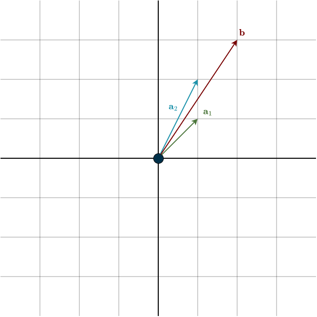
Here, \(\mathbf{a}_1\) and \(\mathbf{a}_2\) denote the respective columns of \(A\). The question is: how much of \(\mathbf{a}_1\) and how much of \(\mathbf{a}_2\) do we need to combine in order to produce \(\mathbf{b}\)?
So how do we actually start solving this? Recall the equation from before:
\(A\mathbf{x} = \mathbf{b}\)
Couldn’t we just “move” the matrix \(A\) to the right by multiplying both sides on the left by its inverse?
\(\mathbf{x} = A^{-1}\mathbf{b}\)
In principle, this works, and it highlights something important. The matrix \(A\) represents a linear transformation, a certain movement of vectors. Its inverse, \(A^{−1}\), undoes that transformation. Multiplying \(\mathbf{b}\) by \(A^{−1}\) gives us \(\mathbf{x}\), which you can think of as the vector \(\mathbf{b}\) before the transformation. From the opposite perspective, \(\mathbf{b}\) is simply the vector \(\mathbf{x}\) after the transformation.
However, not every matrix is invertible, so a solution is not always guaranteed. Even when an inverse does exist, explicitly forming it is usually unnecessary and inefficient. In practice, instead of computing \(A^{−1}\), we solve the system directly using Gaussian elimination.
Gaussian Elimination
The idea behind Gaussian elimination is pretty simple: we want to reshape the matrix \(A\) into a form that’s easy to work with. That form is called an upper triangular matrix, and once we get there, solving the system becomes almost mechanical using something called backward substitution.
So what does “upper triangular” actually mean? Imagine drawing a diagonal line from the top-left corner of the matrix to the bottom-right. In an upper triangular matrix, everything below that line is zero. The diagonal itself stays, and anything above it can be whatever it wants:
\(
\begin{bmatrix}
x & x & x\\
0 & x & x\\
0 & 0 & x\\
\end{bmatrix}
\)
If you look at it this way, the name makes sense, the nonzero entries form a triangle in the upper half of the matrix. Why do we care about this shape? Because it makes solving the system easy. You start at the bottom row, solve for one variable, then move upward, plugging that value into the rows above. Step by step, the whole solution falls into place. I’ll show exactly how this works in the next chapter.
So the real question now is: how do we actually turn the original matrix \(A\) into this upper triangular form?
Let’s walk through a concrete example. Suppose we start with the matrix \(A\):
\(A =
\begin{bmatrix}
1 & 1 & 2\\
2 & 4 & 6\\
3 & 4 & 8\\
\end{bmatrix}
\)
We begin in the top-left corner, with the entry \(a_{11}\). In this case, it’s the number \(1\). This is our pivot, the value we’ll use to eliminate the numbers below it. It cannot be zero.
\(
\begin{bmatrix}
\color{red}{1} & 1 & 2\\
2 & 4 & 6\\
3 & 4 & 8\\
\end{bmatrix}
\)
Now look straight down that first column. Everything below the pivot needs to become zero. So our task is to eliminate the entries in the second and third rows of this column. To eliminate the entry in row 2, column 1, we compute a multiplier:
\(l_{21} = \frac{a_{21}}{a_{11}}\)
It’s called \(l_{21}\) because we’re eliminating the entry in row \(2\) using the pivot in column \(1\). In plain terms, this number tells us how much of row \(1\) we need to subtract from row \(2\) to cancel out the first entry. We always subtract.
\(\text{row 2} = \text{row 2} \; – \; l_{21} \cdot \text{row 1}\)
Here, \(l_{21} = \frac{2}{1} = 2\). So we subtract two times row \(1\) from row \(2\). Remember: the multiplier applies to the entire row, not just the pivot. After doing that, the matrix becomes:
\(
\begin{bmatrix}
\color{red}{1} & 1 & 2\\
0 & 2 & 2\\
3 & 4 & 8\\
\end{bmatrix}
\)
Perfect, the first entry in row \(2\) is now zero. We repeat the same idea for row \(3\). The multiplier is
\(l_{31} = \frac{3}{1} = 3\)
Subtracting three times row \(1\) from row \(3\) gives:
\(
\begin{bmatrix}
\color{red}{1} & 1 & 2\\
0 & 2 & 2\\
0 & 1 & 2\\
\end{bmatrix}
\)
At this point, everything below the first pivot is zero, so we move on. To find the next pivot, we move one step down and one step to the right. The new pivot is \(a_{22}\):
\(
\begin{bmatrix}
1 & 1 & 2\\
0 & \color{red}{2} & 2\\
0 & 1 & 2\\
\end{bmatrix}
\)
This pivot must not be zero, otherwise we’d be dividing by zero when computing the multiplier, which is a big mathematical no-no. Now we eliminate the entry below this pivot. The multiplier is:
\(l_{32} = \frac{1}{2}\)
Subtracting \(\frac{1}{2}\) times row \(2\) from row \(3\) gives:
\(
\begin{bmatrix}
1 & 1 & 2\\
0 & \color{red}{2} & 2\\
0 & 0 & 1\\
\end{bmatrix}
\)
We move the pivot one last time, but there are no rows below it, so we’re done. The original matrix \(A\) has now been transformed into an upper triangular matrix:
\(\begin{bmatrix}
1 & 1 & 2\\
0 & 2 & 2\\
0 & 0 & \color{red}{1}\\
\end{bmatrix}
\)
\( U =
\begin{bmatrix}
1 & 1 & 2\\
0 & 2 & 2\\
0 & 0 & 1\\
\end{bmatrix}
\)
We call this matrix \(U\), for upper triangular.
Why Does This Work?
At this point, you might be wondering: aren’t we changing the system by doing all this elimination? Why should the solution stay the same after all these steps? That’s a completely fair question. To see why this works, notice that elimination is really just taking linear combinations of the rows.
In fact, every elimination step you’ve seen so far is just a row operation: multiply a row by a number and subtract it from another row. And there’s a clean way to describe all of this using matrices. When we multiply a matrix on the left, we are taking linear combinations of its rows. So each elimination step can be written as a matrix multiplication using what are called elimination matrices.
Let’s go back to our matrix \(A\) and look at the very first elimination step. We eliminated the entry below the first pivot using the multiplier \(l_{21}=2\). That step can be written as:
\(E_{21}A = \begin{bmatrix} 1 & 0 & 0 \\ -l_{21} & 1 & 0 \\ 0 & 0 & 1\end{bmatrix} \begin{bmatrix} 1 & 1 & 2\\ 2 & 4 & 6\\ 3 & 4 & 8\\ \end{bmatrix} =\begin{bmatrix} 1 & 0 & 0 \\ -2 & 1 & 0 \\ 0 & 0 & 1\end{bmatrix} \begin{bmatrix} 1 & 1 & 2\\ 2 & 4 & 6\\ 3 & 4 & 8\\ \end{bmatrix} = \begin{bmatrix} 1 & 1 & 2\\ 0 & 2 & 2\\ 3 & 4 & 8\\ \end{bmatrix} \)
If you look closely, you can actually read this multiplication row by row.
- The first row of \(E_{21}\) just says: “take the first row of \(A\) as it is.”
- The second row says: “take the first row of \(A\), multiply it by \(−2\), and add it to the second row.” That’s exactly the elimination step we performed earlier.
- The third row simply copies the third row of \(A\).
So nothing mysterious is happening here, we’re doing the same row operations as before, just written in matrix form. Another nice detail is how easy these elimination matrices are to build. You start with the identity matrix of the right size and place the negative multiplier in the appropriate position. The subscript in \(E_{21}\) and \(l_{21}\) tells you exactly where it goes. If we keep doing this for every elimination step, the entire Gaussian elimination process can be written compactly as:
\(U = E_{32}E_{31}E_{21}A\)
The order matters. \(E_{21}\) acts first, then \(E_{31}\), then \(E_{32}\), just like we saw earlier when discussing matrix multiplication. The key reason all of this works is that elimination matrices are invertible. That fact is what guarantees we don’t change the solution when we apply them. Here’s what that means in practice. Start with the original system:
\(A\mathbf{x} = \mathbf{b}\)
If we multiply both sides on the left by an elimination matrix \(E\), we get:
\(A\mathbf{x} = \mathbf{b} \hspace{0.5cm} \Rightarrow \hspace{0.5cm} EA\mathbf{x} = E\mathbf{b}\)
Written this way, it looks like we’ve only moved in one direction, from the original system to a new one. But for the two systems to truly be equivalent, we need to be able to go back as well. That’s where invertibility comes in. Since \(E\) is invertible, we can undo the transformation:
\(EA\mathbf{x} = E\mathbf{b} \hspace{0.5cm} \Rightarrow \hspace{0.5cm} E^{-1}EA\mathbf{x} = E^{-1}E\mathbf{b} \hspace{0.5cm} \Rightarrow \hspace{0.5cm} IA\mathbf{x} = I\mathbf{b} \hspace{0.5cm} \Rightarrow \hspace{0.5cm} A\mathbf{x} = \mathbf{b}\)
So multiplying by \(E\) doesn’t lose any information, it’s completely reversible. If \(E\) were not invertible, this step would fail, and we would no longer be guaranteed that the solution stays the same. Because of this, we can safely say:
\(A\mathbf{x} = \mathbf{b} \hspace{0.5cm} \Leftarrow \hspace{0.5cm} EA\mathbf{x} = E\mathbf{b}\)
and therefore,
\(A\mathbf{x} = \mathbf{b} \hspace{0.5cm} \Leftrightarrow \hspace{0.5cm} EA\mathbf{x} = E\mathbf{b}\)
In other words, both systems have exactly the same solution. The vector \(\mathbf{x}\) doesn’t change at all, we’ve only rewritten the equations in a more convenient form. The vectors, that is, the columns of \(A\) and the right-hand-side vector \(\mathbf{b}\), may look different, but the underlying solution is the same.
Keep in mind that whenever you apply elimination steps to \(A\), you must apply the same steps to \(\mathbf{b}\) as well, otherwise, the solution will be incorrect. I’m not stressing this too much here because we’ll handle elimination a bit differently in the next chapter. For now, the goal is simply to focus on the coefficient matrix \(A\) and get comfortable with performing elimination on it.
What the Pivot Tells Us
As mentioned earlier, a pivot cannot be zero, since division by zero is undefined. So if we run into a zero where a pivot is supposed to be, we simply don’t treat it as one. What can we do in such a situation? There are two possibilities.
First, the easy case: the pivot is there, just not in the right place. Often this can be fixed by reordering the rows. For example, take the matrix
\(\begin{bmatrix}
0 & 1 & 2\\
1 & 4 & 3\\
0 & 0 & 7\\
\end{bmatrix}\)
At first, the top-left entry is zero, which looks like a problem. But if we swap the first two rows, the issue disappears:
\(\begin{bmatrix}
1 & 4 & 3\\
0 & 1 & 2\\
0 & 0 & 7\\
\end{bmatrix}\)
Now everything is fine, and we can continue with elimination as usual.
Second case: the zero pivot cannot be fixed by row swaps.
This situation is more serious. Recall that Gaussian elimination consists of taking linear combinations of rows. If, during elimination, we end up with a zero in a pivot position that cannot be removed by row exchanges, this reveals something fundamental: linear dependence. One row is a linear combination of the previous rows, meaning the rows are linearly dependent and the matrix is singular. The same idea applies to the columns. If the rows are dependent, then the columns are dependent too. These two perspectives go hand in hand. Consider the following matrix:
\(\begin{bmatrix} 1 & 2 & 3 \\ 2 & 4 & 6 \\ 3 & 6 & 9 \\ \end{bmatrix}\)
Here, the dependence jumps out right away. The second column is just twice the first, and the third column is three times the first. The same pattern appears in the rows as well, each row is a multiple of the first one. If we run Gaussian elimination, this dependence shows up automatically. After elimination, the matrix becomes
\(\begin{bmatrix} 1 & 2 & 3 \\ 0 & 0 & 0 \\ 0 & 0 & 0 \\ \end{bmatrix}\)
The zero rows, and in particular the missing pivots, tell us exactly what’s going on: there’s only one independent row (and one independent column). This is a very simple example where the dependence is obvious at a glance. But the important point is that even when the dependence isn’t so easy to spot, elimination will always uncover it for us.
Whether a singular matrix still has solutions depends on its shape and its rank. We’ll look at what those solutions look like shortly. Pivots tell us which columns are linearly independent. These columns form a basis for the column space of the matrix. Consequently, the number of pivots equals the rank of the matrix, since the rank is defined as the dimension of the column space, and the dimension is given by the number of basis vectors. If the number of pivots equals \(n\), the matrix has full rank if it is square, or full column rank if it is rectangular. In short:
\(\text{number of pivots} = \text{rank}\)
Important Note: Gaussian elimination will detect singularity, but it cannot proceed once singularity is encountered, since the pivot positions contain only zeros and division by zero is not possible. This means that only square, invertible matrices can be solved using this process alone. There are other ways to solve \(A\mathbf{x}=\mathbf{b}\) when \(A\) is singular, such as least squares or the pseudoinverse, which we will cover in future chapters.
How Many Solutions Does the System Have?
The number of solutions a linear system has depends on the shape of the matrix that represents it and the rank of that matrix. Recall that solving the system
\(A\mathbf{x} = \mathbf{b}\)
means finding coefficients such that a linear combination of the columns of \(A\) produces the vector \(\mathbf{b}\). In other words, a solution exists if and only if \(\mathbf{b}\) lies in the column space of \(A\) (span of the columns of \(A\)). By the definition of span, if \(b\) is in the column space, then there must exist at least one linear combination of the columns of \(A\) that equals \(\mathbf{b}\), this linear combination is our solution. However, this solution is not necessarily unique. If the columns of \(A\) are linearly dependent, multiple different combinations can produce the same vector \(\mathbf{b}\), leading to infinitely many solutions.
We can categorize the behavior of linear systems into four distinct cases. Consider the first case:
Case 1: m > n and full column rank
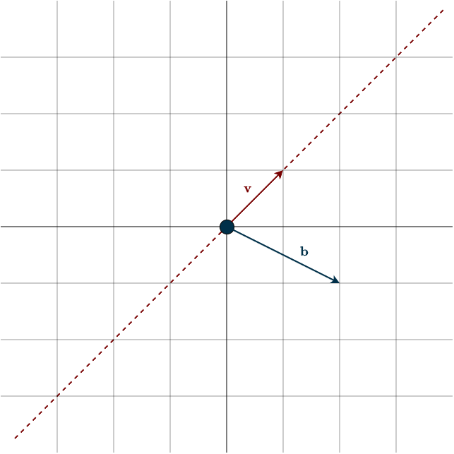
Here, \(A\) is a tall matrix, meaning it has more rows than columns. Having full column rank implies that the columns of \(A\) are linearly independent. As a result, the null space contains only the zero vector, so any solution, if it exists, is unique. However, while the columns are independent, they do not span the entire output space \(\mathbb{R}^m\). Instead, they span only an \(n\)-dimensional subspace inside a higher-dimensional space. Geometrically, this is like embedding a lower-dimensional object into a higher-dimensional space.
A helpful analogy is a sheet of paper floating in 3D space (look at figure below). No matter how you rotate it, the paper cannot fill the entire 3D space, there will always be points above and below it that the paper never touches. Similarly, the column space of \(A\) does not span all of \(\mathbb{R}^m\). As a consequence, the vector \(\mathbf{b}\) may or may not lie in the column space of \(A\):
- If \(\mathbf{b}\) is not in the column space, the system has no solution.
- If \(\mathbf{b}\) is in the column space, the system has exactly one unique solution.
Looking at the figure below, we see that b is not in the column space (dotted line) of v, and therefore there is no solution.
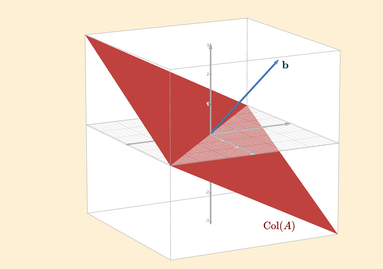
Similarly, we could have a two-dimensional column space in \(\mathbb{R}^3\). Again, the right-hand side vector \(\mathbf{b}\) is not in the column space, so there is no solution.
Case 2: m < n and full row rank
Here, \(A\) is a wide matrix. If \(A\) has full row rank, then \(\text{rank}(A)=m\). Since the row rank equals the column rank, the column space of \(A\) spans the entire output space \(\mathbb{R}^m\). As a result, the right-hand side vector \(\mathbf{b}\) must lie in the column space of \(A\). It cannot hide. Therefore the linear system \(A\mathbf{x}=\mathbf{b}\) is always solvable.
However, since there are more columns than rows, the matrix contains more vectors than are needed to span \(\mathbb{R}^m\). Consequently, the columns of \(A\) are linearly dependent. This linear dependence implies that the solution to \(A\mathbf{x}=\mathbf{b}\) cannot be unique. Instead, the system has infinitely many solutions.
Remember that only two vectors are needed to form a basis for a two-dimensional space. If we introduce a third vector, it must lie in the span of the first two and is therefore redundant. Consider the example
\(A = \begin{bmatrix} 1 & 3 & 4\\ 2 & 7 & 9 \\ \end{bmatrix}\)
Suppose we want to express the vector \(\mathbf{b}=(4,9)\) as a linear combination of the columns of \(A\). One obvious choice is
\(0 \cdot \mathbf{a}_1 + 0 \cdot \mathbf{a}_2 + 1 \cdot \mathbf{a}_3 = 0 \cdot \begin{bmatrix} 1 \\ 2 \end{bmatrix} + 0 \cdot \begin{bmatrix} 3 \\ 7 \end{bmatrix} + 1 \cdot \begin{bmatrix} 4 \\ 9 \end{bmatrix} = \begin{bmatrix} 4 \\ 9 \end{bmatrix}\)
But this is far from the only option. We could just as well use
\(1 \cdot \mathbf{a}_1 + 1 \cdot \mathbf{a}_2 + 0 \cdot \mathbf{a}_3 = 1 \cdot \begin{bmatrix} 1 \\ 2 \end{bmatrix} + 1 \cdot \begin{bmatrix} 3 \\ 7 \end{bmatrix} + 0 \cdot \begin{bmatrix} 4 \\ 9 \end{bmatrix} = \begin{bmatrix} 4 \\ 9 \end{bmatrix}\)
or even
\(2 \cdot \mathbf{a}_1 + 2 \cdot \mathbf{a}_2 \;- 1 \cdot \mathbf{a}_3 = 2 \cdot \begin{bmatrix} 1 \\ 2 \end{bmatrix} + 2 \cdot \begin{bmatrix} 3 \\ 7 \end{bmatrix} -1 \cdot \begin{bmatrix} 4 \\ 9 \end{bmatrix} = \begin{bmatrix} 4 \\ 9 \end{bmatrix}\)
and many other combinations. Because the third column is redundant, at least one variable is free, allowing us to adjust the coefficients while still producing the same vector \(\mathbf{b}\). In summary, when \(A\) is wide and has full row rank, the system \(A\mathbf{x}=\mathbf{b}\) has infinitely many solutions.
Case 3: m = n and full rank
Here we are considering square, invertible matrices, which represent the ideal case. The columns span the entire output space which means that every possible vector can be reached. At the same time, there are exactly as many columns as needed, no more, no less, so there is no redundancy. In other words, the columns form a basis. Because of this, the solution is unique. This case combines the properties of the previous scenarios: full coverage without redundancy.
As a result, for every possible right-hand side vector \(\mathbf{b}\), there exists exactly one unique solution.
Case 4: General case — neither full column rank nor full row rank
Because the matrix does not have full column rank, its columns are linearly dependent, so any solution, if it exists, will not be unique. Additionally, since the matrix does not have full row rank, its column space does not span the entire output space, which means that for some right-hand side vectors there may be no solution at all.
Note that this is not because the rows fail to span the output space. The rows span a subspace of the input space. The reason full row rank implies that the column space spans the output space is because \(\text{row rank} = \text{column rank}\). Specifically:
\(\text{not full row rank} \hspace{0.5cm} \Rightarrow \hspace{0.5cm} \text{rank}(A) < m \hspace{0.5cm} \Rightarrow \hspace{0.5cm} \text{dim}(\text{Col}(A)) < m \hspace{0.5cm} \Rightarrow \hspace{0.5cm} \text{Col}(A) \neq \mathbb{R}^m\)
where \(\text{Col}(A)\) denotes the column space of \(A\).
In summary, this case leads to either infinitely many solutions or no solution, depending on the right-hand side vector \(\mathbf{b}\).
In theory, we could find these infinitely many solutions and construct the complete solution to \(A\mathbf{x}=\mathbf{b}\), instead of taking just one particular solution (see the references for more information. In essence this involves solving for the basis of the nullspace). In practice, however, in a machine learning context, problems are formulated explicitly so that a single, stable solution exists, usually involving an invertible matrix. This is why I will not include an explanation of how to compute the other solutions here.
How Much Metal Does Each Android Cost?
We now know enough to finish the example we started at the beginning of the chapter. Let’s quickly recall the system:
\(\begin{bmatrix} 1 & 1 \\ 1 & 2 \end{bmatrix} \begin{bmatrix} x \\ y \end{bmatrix} = \begin{bmatrix} 2 \\ 3 \end{bmatrix}\)
Using elimination (remember that every row operation must also be applied to the right-hand side vector), we get:
\(\begin{bmatrix} 1 & 1 \\ 0 & 1 \end{bmatrix} \begin{bmatrix} x \\ y \end{bmatrix} = \begin{bmatrix} 2 \\ 1 \end{bmatrix}\)
We now apply backward substitution to solve for the variables. I will explain this method in detail in the next chapter, but the idea is simple: the last row is already solved. From it, we immediately get
\(y = 1\)
Next, we substitute this value into the equation in the row above. This leaves us with a single unknown, which we can solve easily:
\(x + y = 2 \hspace{0.5cm}\Rightarrow \hspace{0.5cm} x + 1 = 2 \hspace{0.5cm} \Rightarrow \hspace{0.5cm} x = 1\)
Therefore, the final solution vector is
\(\mathbf{x} = \begin{bmatrix} 1 \\ 1\end{bmatrix}\)
This means that both androids use the same amount of metal, specifically, 100 kg each. You can also see this visually in the figure below
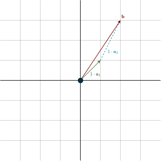
Below is a figure visualizing the columns of \(A\) and the right-hand-side vector \(\mathbf{b}\) after the elimination, denoted by the * symbol. Notice that although the vectors look different, the solution is the same. The combination remains unchanged.
Each step of Gaussian elimination changes how the vectors look, but the solution, meaning the correct linear combination, remains unchanged.
Summary
- A linear equation is an equation in which each variable has power 1, variables are multiplied by constants, and variables are combined only through addition.
- A system of linear equations consists of multiple linear equations solved simultaneously.
- A linear system can be written in matrix form as \(A\mathbf{x}=\mathbf{b}\). Solving the system means finding a vector \(\mathbf{x}\) such that a linear combination of the columns of \(A\) equals the vector \(\mathbf{b}\).
- Systems of linear equations are solved systematically using Gaussian elimination. It is only possible when \(A\) is a square, invertible (non-singular) matrix.
- During Gaussian elimination, each pivot corresponds to an independent direction, the number of pivots equals the rank of the matrix, and if a pivot position contains a zero, we attempt to fix it using row swaps; if it cannot be fixed, the matrix is singular.
- Gaussian elimination can be represented using matrix multiplication with elimination matrices. Elimination does not change the solution set: the rows and vectors may change, but the underlying linear combinations remain the same.
- The existence and uniqueness of solutions depend on the size and rank of \(A\).
- If \(A\) has \(m > n\) and full column rank, there is either one unique solution or no solution, depending on whether \(\mathbf{b}\) lies in the column space of \(A\).
- If \(A\) has \(m < n\) and full row rank, there are infinitely many solutions for every \(\mathbf{b}\), the solutions are not unique.
- If \(A\) has \(m = n\) and full rank, then \(A\) is invertible, and a unique solution exists for every \(\mathbf{b}\).
- In all other cases, the system has either no solution or infinitely many solutions, depending on whether \(\mathbf{b}\) lies in the column space of \(A\).