Linear Transformations

Up to this point, we’ve focused on how new vectors can be formed from existing ones through linear combinations. We’ve seen that vectors can be linearly dependent, (some vectors are essentially redundant) and we’ve explored how different collections of vectors (subspaces) can be combined to form larger ones, sometimes even spanning the entire vector space. But throughout all of this, the vectors themselves never moved; we only described how they could be constructed and how they relate to one another.

Now imagine we want to do something different: we want to move vectors. To do that, we need some kind of machine, an operation that takes in a vector, determines where it should go, and outputs the resulting vector.

We call this machine a transformation. More specifically, we will focus on linear transformations, which we will denote by \(T\). For any input vector \(\mathbf{v}\), the expression \(T(\mathbf{v})\) represents the output vector produced by the transformation.

Geometrically, a transformation is linear if it preserves the structure of the grid: parallel lines remain parallel, evenly spaced lines remain evenly spaced, lines map to lines, and shapes like triangles maintain their straight edges (though they may be stretched, squashed, or rotated). Points that were equally spaced remain equally spaced, and the origin stays fixed.

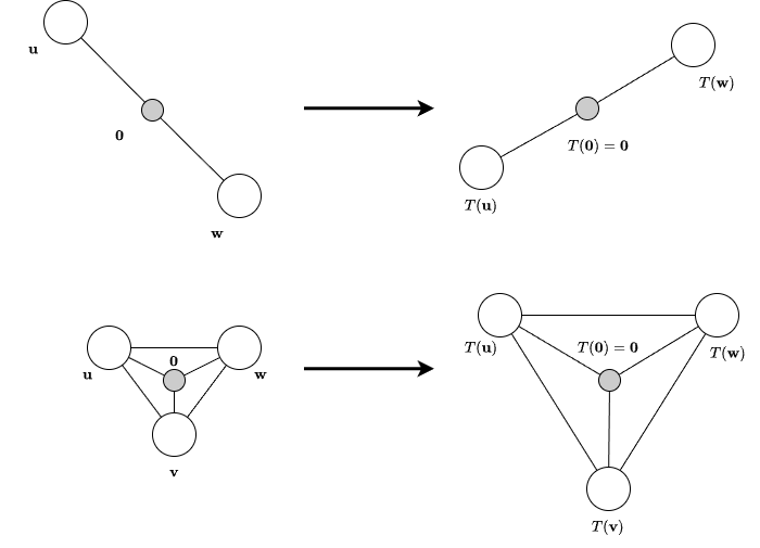
Think of the following analogy to make linearity more intuitive. Imagine you have two 50 € bills that you want to convert to US dollars. Suppose the exchange rate is 1.2. The bills represent vectors, and the currency exchange represents a linear transformation. You could convert each 50 € bill separately. Each one becomes 60 $, giving a total of 120 $. Alternatively, you could first add the two bills together to get 100 €, and then convert that amount directly, again obtaining 120 $. In both cases, the result is the same. In linear algebra terms, this means that the transformation of a sum equals the sum of the transformations.

The same idea applies when you scale the amount of euros by some number. If you double your money, the dollar amount also doubles; if you triple it, the dollar amount triples as well. In other words, multiplying the input by a number multiplies the output by that exact same number. Now think about this geometrically. Amounts like 10 €, 20 €, 30 €, and so on are evenly spaced. After applying the conversion, they become 12 $, 24 $, 36 $, etc. The exact distances change (\(10 \neq 12\)), but the spacing remains uniform. This is the key idea behind linearity: a linear transformation may scale or stretch space, but it preserves relative structure. Equal steps in the input remain equal steps in the output.

Mathematically, linearity means that the transformation cannot involve operations such as taking powers, roots, logarithms, lengths, or products of coordinates.

How exactly does a linear transformation work? First, we need to know where the input vector lives, that is, the vector space it comes from. We call this the input vector space, denoted by \(V\).

Here’s where things get interesting: a linear transformation doesn’t just move vectors around within the same space, it can also send them into an entirely different vector space. In other words, the output does not have to live in \(V\); it can land in another space \(W\). A linear transformation is like a portal that takes vectors from one “world,” the space \(V\), and transports them into another, \(W\). Let’s look at the formal definition:

Let’s explore a few examples to develop a clearer understanding. A classic one is shearing a vector to the right: imagine taking hold of the vector’s tip and pulling it to the right while keeping its base fixed:

Here is a short animation illustrating the movement:

Another example is reflecting a vector across an axis, here, across the origin (negating all coordinates). This operation essentially produces a mirror image of the original vector:

Again, here is an animation showing the movement:

Before moving on, let’s look at one final example, which is a bit different. In the previous examples, the input and output spaces were the same, so the vectors stayed within the same space. Now, let’s see what happens when we transform from \(\mathbb{R}^2\) to \(\mathbb{R}\):

Essentially, we only took the first coordinate of the vector. Mathematically, it can be expressed as:

\(T(\mathbf{v}) = T((v_1, v_2)) = (v_1)\)

Notice the difference between \(\mathbb{R}^2\) and \(\mathbb{R}\): \(\mathbb{R}\) is one-dimensional, consisting of only a line of vectors (or numbers, i.e., the number line). There are no other directions or dimensions. You might ask, what happened to the second dimension? In this transformation, we only keep the first coordinate and ignore the second, essentially throwing it out the window. In other words, we lose information. Transformations like these are very important and will be discussed explicitly later. They are referred to as singular or non-invertible.

In this course, we primarily work with the vector space \(\mathbb{R}^n\), but vector spaces are abstract and can take many forms, as we saw in the first chapter. Remember that the set of polynomials of degree 3 or less forms a vector space. This means we can create a linear transformation between \(\mathbb{R}^4\) and that vector space. Here is an example:

\(T(\mathbf{v}) = T((v_1, v_2, v_3, v_4)) = v_1 \cdot x^3 + v_2 \cdot x^2 + v_3 \cdot x + v_4 \)

This example emphasizes that we can, in principle, map from any vector space to any other vector space, as long as the transformation remains linear and the dimensions match.

These illustrations of moving vectors are fun and all, but how do we actually construct a linear transformation? How can we determine where the vectors in the examples above will end up after the transformation? And if we know how, do we need to apply the transformation every time we want to see where a specific vector goes?

Basis Tells It All

Imagine you have a linear transformation \(T: V \rightarrow W\), and you choose a basis of the input space

\((\mathbf{v}_1, \dots ,\mathbf{v}_n)\)

By definition, a basis must span the vector space, meaning every vector in \(V\) can be reached, and must be linearly independent, meaning every vector has a unique representation in terms of the basis vectors. Therefore, any vector \(\mathbf{x} \in V\) can be uniquely written as:

\(\mathbf{x} = a_1 \cdot \mathbf{v}_1 + \dots + a_n \cdot \mathbf{v}_n\)

Now, because \(T\) is linear, it preserves linear combinations. So when we apply \(T\) to \(\mathbf{x}\), we get

\(T(\mathbf{x}) = T(a_1 \cdot \mathbf{v}_1 + \dots + a_n \cdot \mathbf{v}_n)\)

Using additivity, this becomes:

\(T(\mathbf{x}) = T(a_1 \cdot \mathbf{v}_1) + \dots + T(a_n \cdot \mathbf{v}_n)\)

and pulling out the scalars gives:

\(T(\mathbf{x}) = a_1 \cdot T(\mathbf{v}_1) + \dots + a_n \cdot T(\mathbf{v}_n)\)

This shows something powerful: Knowing only the transformed basis vectors \(T(\mathbf{v}_1), \dots, T(\mathbf{v}_n)\) completely determines the entire transformation \(T\). Every possible output \(T(\mathbf{x})\) is just the corresponding linear combination of those transformed basis vectors.

(Note that once you choose a basis for the input and output vector spaces, the linear transformation described in terms of those bases is unique. Given those bases, there is no other transformation that produces the same action. However, a linear transformation can have many different descriptions depending on which bases you choose. Changing the basis changes how the transformation looks, even though the underlying transformation itself stays the same.)

You can also describe a linear transformation in the abstract mathematical sense. For example:

\(T(\mathbf{v}) = T((v_1, v_2)) = (-v_1, -v_2) = -\mathbf{v}\)

This transformation reflects a vector across the origin. But in the context of machine learning, we usually don’t work with linear transformations in this abstract sense. Instead, we choose a basis (most often the standard basis) and describe vectors directly using their coordinates in that basis. Linear transformations are then understood with respect to that chosen basis. Let’s look at an example so you can see what I mean.

Example (standard basis)

Suppose \(V = \mathbb{R}^2\) and \(\mathbf{v} = (2,3)\), and let our linear transformation be a 90° clockwise rotation. Because this transformation simply rotates vectors in the plane, the input and output vector spaces are the same, and we use the same basis for both, in this case, the standard basis.
With respect to this basis, the vector \(\mathbf{v}\) can be written as the linear combination:

\(\mathbf{v} = 2 \cdot \mathbf{\hat{i}} + 3 \cdot \mathbf{\hat{j}}\)

To compute \(T(\mathbf{v})\), we only need to apply the transformation to the basis vectors. This gives us the following linear combination:

\(T(\mathbf{v}) = 2 \cdot T(\mathbf{\hat{i}}) + 3 \cdot T(\mathbf{\hat{j}}) = 2 \cdot \begin{bmatrix} 0\\ -1\\ \end{bmatrix} + 3 \cdot \begin{bmatrix} 1\\ 0\\ \end{bmatrix} = \begin{bmatrix} 3\\ -2\\ \end{bmatrix}\)

Important Note: Coordinates are just scalars, numbers that tell you how much to scale each basis vector. The basis vectors themselves are what define the coordinate system. So if you are given a vector like \(\mathbf{v} = (2,3)\), those numbers are meaningless until you know which basis they refer to. Which vector is being scaled by \(2\)? Which is being scaled by \(3\)? Without the basis, the coordinates tell you nothing.

Now for the crucial point: \(T(\mathbf{v})\) lives in the output space. Remember: A linear transformation is a mapping from one vector space to another: it takes a vector from the input space \(V\) (the domain) and sends it to a corresponding vector in the output space \(W\) (the codomain). Each vector space comes equipped with its own basis, and any vector in these spaces must be expressed in terms of its respective basis to work with the transformation properly.

In the earlier example, the input and output bases were both the standard basis, but this does not have to be the case. The output space might use a completely different basis, or even be a different vector space altogether. This means the coordinate representation of \(T(\mathbf{v})\) must be expressed using the basis of the output space; otherwise, the resulting coordinates would have no meaning within that space.

If the output space \(W\) uses a different basis, then we must rewrite the vector we computed in terms of that basis. Suppose the basis of \(W\) is \((\mathbf{w}_1, \dots, \mathbf{w}_m).\) Then we need to find scalars \(b_1, \dots, b_m\)​ such that:

\(T(\mathbf{v}) = b_1 \cdot \mathbf{w}_1 + \dots + b_m \cdot \mathbf{w}_m\)

These coefficients give the coordinates of \(T(\mathbf{v})\) in the output basis, completing the representation. (Solving for these coefficients can be done either by solving a system of linear equations or by using a change-of-basis matrix.)

To make this concrete, let’s consider an example where the output basis is not the standard basis.

Example (different bases)

Let the input vector space be \(V = \mathbb{R}^2\) with the standard basis, and let the output vector space also be \(\mathbb{R}^2\), but equipped with a different basis:

\(\mathbf{w}_1 = \begin{bmatrix} 1\\ 1\\ \end{bmatrix}, \hspace{1cm} \mathbf{w}_2 = \begin{bmatrix} 1\\ -1\\ \end{bmatrix}\)

Note that the coordinates written for these basis vectors are expressed with respect to the standard basis. In their own basis, however, these vectors would look exactly like the standard basis looks in the standard coordinate system:

\(\mathbf{w}_1 = \begin{bmatrix} 1\\ 0\\ \end{bmatrix}, \hspace{1cm} \mathbf{w}_2 = \begin{bmatrix} 0\\ 1\\ \end{bmatrix}\)

I know this is confusing at first but stick with me here. The input vector remains the same, which gives us the following linear combination:

\(T(\mathbf{v}) = 2 \cdot T(\mathbf{\hat{i}}) + 3 \cdot T(\mathbf{\hat{j}}) = \begin{bmatrix} 3\\ -2\\ \end{bmatrix}\)

Now, focus on the left subfigure above and compare it with the figure at the top of this section. Our goal is to express \(T(\mathbf{v})\) using only \(\mathbf{w}_1\)​ and \(\mathbf{w}_2\)​. At this point, it’s clear that the coordinates we currently have are incorrect (scaling \(\mathbf{w_1}\) by \(3\) and \(\mathbf{w_2}\) by \(2\), then adding the results, would produce a vector lying in the upper-right quadrant, whereas \(T(\mathbf{v})\) should lie in the quadrant directly below it.), because they are still expressed with respect to the standard basis. To fix this, we need to convert them to the output basis. By solving for the coordinates in the output basis, we obtain the following result:

\([T(\mathbf{v})]_{B_W} = \begin{bmatrix} \frac{1}{2}\\ \frac{5}{2}\\ \end{bmatrix}\)

The subscript \(B_W\)​ indicates that the vector’s coordinates are expressed with respect to the basis of the output space \(W\).

It is also possible to express \(T(\mathbf{\hat{i}})\) and \(T(\mathbf{\hat{j}})\) directly in the output basis. If you do this, then forming linear combinations of these transformed basis vectors will automatically give you the correct expression for \(T(\mathbf{v})\) in that basis.

However, most textbook and university exercises provide vectors in the standard basis, because it is the one we are most familiar with. As a result, you usually need to convert those vectors into the appropriate basis before applying the transformation, or alternatively, apply the transformation in the standard basis and then convert the result into the desired basis, as we did above.

In the figure below, you can see how \(\mathbf{v}\) and \(T(\mathbf{v})\) are expressed using the output basis vectors. The left subfigure shows these vectors from the perspective of the standard basis, while the right subfigure shows how \(\mathbf{v}\) and \(T(\mathbf{v})\) appear in the coordinate system defined by the output basis itself. The green and blue arrows represent the basis vectors that span each coordinate system.

Notice that the two coordinate systems are simply rotated versions of one another, specifically by 45°. This is just a convenient choice for visualization. In general, a basis does not need to consist of perpendicular vectors or correspond to a rotation of the standard basis; this example was selected purely because it makes the geometry easier to see.

Now that we understand how to define and describe a single linear transformation, we can naturally ask whether it is possible to combine multiple movements into one.

Products of Linear Transformations

Consider the set of all linear transformations from a vector space \(V\) to another vector space \(W\), which we denote by \(\mathcal{L}(V, W)\). Within that, we can formally define the product (that is, the composition) of linear transformations:

The product \(ST\) is simply the composition of functions: you apply one transformation to a vector, then take the result and feed it into the other. This composition is read from right to left, since the rightmost transformation is applied first.

For the product \(ST\) to be well-defined, the vector spaces must line up correctly. In particular, the codomain of \(T\) must match the domain of \(S\). More precisely, \(ST\) is defined only when

\(T: V \rightarrow U\) and \(S: U \rightarrow W\)

so that the output of \(T\) can be used as the input of \(S\). If the spaces do not match, the product is undefined.

For example, if

\(T: \mathbb{R}^3 \rightarrow \mathbb{R}^2\) and \(S: \mathbb{R}^3 \rightarrow \mathbb{R}^3\)

then the product \(ST\) cannot be formed, because the codomain of \(T\) (\(\mathbb{R}^2\)) does not match the domain of \(S\) (\(\mathbb{R}^3\)).

The product of linear transformations satisfies the familiar algebraic properties:

However, there is a crucial exception: the product of linear transformations is not commutative.

\(ST(\mathbf{u}) \neq TS(\mathbf{u})\)

The order in which you apply transformations matters, and changing the order generally changes the result. For example, performing a rightward shear (\(T\)) followed by a 90° clockwise rotation (\(S\)) is not the same as first rotating 90° clockwise and then applying the shear.

The figure above illustrates the meaning of the product of linear transformations: it represents applying several transformations in sequence, but treating the entire sequence as a single combined transformation.

So if you have a product like \(RTS(\mathbf{v})\), this means the vector \(\mathbf{v}\) is first transformed by \(S\), then the result is transformed by \(T\), and finally by \(R\). The product encapsulates this entire sequence into one seamless, continuous operation.

Summary

• Linear transformations are about moving vectors around, either from one vector space to another, or within the same vector space.
• To fully determine a linear transformation, it is enough to know how the basis vectors are transformed.
• These transformed basis vectors must be written in terms of the basis of the output space, since that is the space they belong to.
• The product of linear transformations corresponds to applying each transformation sequentially, but treating the result as one smooth combined action.
• The order of this sequence matters, since the product is not commutative, and the composition only makes sense when the vector spaces involved match correctly.