Vectors, Span and Basis

On the previous page, we examined the vector space \(\mathbb{R}^n\) from a purely mathematical point of view. While that definition is precise, it is also quite abstract and does little to build intuition for the machine learning algorithms we will study later. In this section, we will connect geometric vectors to vectors in \(\mathbb{R}^n\), that is, to lists of numbers. Along the way, we will introduce several basic but important concepts that follow directly from the definition of a vector space. Let’s begin with vectors.

How Numbers Represent Arrows

Geometric vectors are simply arrows. You may already be familiar with them, and they look like this:

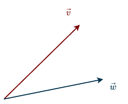
Notice that there is no grid and no numbers attached to these arrows. Even without a coordinate system, we can still work with them. We can add vectors using the tip-to-tail method (see below), and we can scale them (see below) by a number, meaning we can stretch or shrink them, all without ever introducing coordinates or a grid.

We now turn our attention to vectors in \(\mathbb{R}^n\). In the literature, these vectors are typically written using a bold letter, such as \(\mathbf{v}\), and enclosed in parentheses or brackets. Notice that there is no arrow above the letter \(\mathbf{v}\), since an \(\mathbb{R}^n\) vector is a list of numbers rather than a geometric vector. In the vector space \(\mathbb{R}^2\), an example vector might look like this:

\(
\mathbf{v} = \begin{bmatrix}
2\\
3\\
\end{bmatrix}
\)

or generally:

\(
\mathbf{v} = \begin{bmatrix}
v_1\\
v_2\\
\end{bmatrix}
\)

with \(v_1, v_2 \in \mathbb{R}\) and \(\mathbf{v} \in \mathbb{R}^2\). In some textbooks, a vector might also be written in a single line like this: \(\mathbf{v} = (v_1, v_2)\). This is the same list notation we saw on the previous page, both notations mean the same thing.

So how do we connect these two worlds? How can we represent an arrow using numbers?

Imagine you are given 100 different arrows in space and asked to add them all together and draw the resulting vector. Doing this by hand would be tedious and error-prone. Wouldn’t it be much easier to translate those arrows into numbers and let a computer handle the calculations? This is where the idea of a basis comes in. At the bottom of this page, we’ll discuss bases in more detail, but for now, you can think of them as the building blocks that make this translation possible. A basis provides a reference system that allows us to describe geometric vectors using numbers.

Imagine drawing two reference vectors and calling them \(\vec{e}_1\)​ and \(\vec{e}_2\)​. You can place them anywhere you like. For convenience, we will place them in the same directions as the vectors \(\vec{v}\) and \(\vec{w}\).

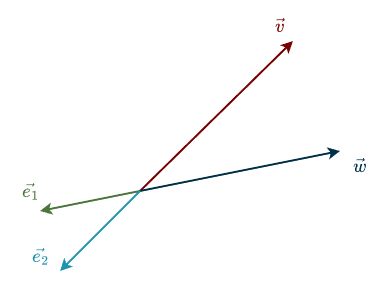
Now we want to add some helpful guide lines to make the visualization clearer. Imagine drawing a line in the direction of \(\vec{e}_1\)​​. Then draw another line parallel to it, shifted by one unit in the direction of \(\vec{e}_2\)​​. Repeat this process several times. Similarly, imagine drawing a line in the direction of \(\vec{e}_2\)​​ and adding more lines parallel to it. Together, these lines form a grid, a coordinate system.

This coordinate system depends entirely on the basis we choose. In fact, the basis defines the coordinate system. Once a basis is fixed, we can assign numbers to geometric vectors. For example, let’s define the basis vectors \(\mathbf{e}_1\)​ and \(\mathbf{e}_2\)​​ as the following vectors in \(\mathbb{R}^2\):

\(\mathbf{e}_1 = \begin{bmatrix} 1 \\ 0\end{bmatrix}, \hspace{0.5cm} \mathbf{e}_2 = \begin{bmatrix} 0 \\ 1\end{bmatrix}\)​

This choice makes sense when you think of basis vectors as defining directions and units. Taking one step in a given direction means moving exactly one basis vector in that direction. You can think of this like some weird measurement system based on the length of your foot. Your foot becomes the reference unit. An object that is two feet long has a length equal to two copies of your foot. Your foot itself has length one because it defines the unit. A basis works the same way, except we have one reference unit for each direction, each represented by one coordinate.

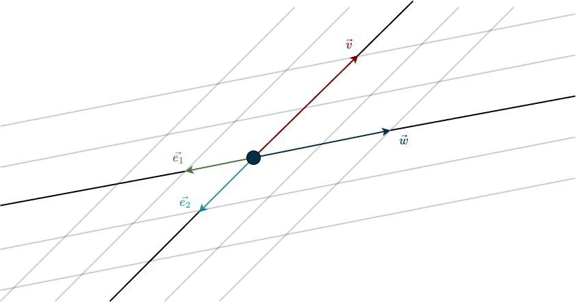
With this basis, the geometric vector \(\vec{v}\) in the figure above can be described as moving twice in the direction opposite to \(\vec{e}_1\)​​. We already reach \(\vec{v}\) without needing any component of \(\vec{e}_2\)​​. Similarly, the geometric vector \(\vec{w}\) can be described by moving twice in the negative \(\vec{e}_2\)​​ direction, with no contribution from \(\vec{e}_1\)​​. This gives

\(\mathbf{v} = -2 \cdot \mathbf{e}_1 + 0 \cdot \mathbf{e}_2 = -2 \cdot \begin{bmatrix} 1 \\ 0 \end{bmatrix} + 0 \cdot \begin{bmatrix} 0 \\ 1 \end{bmatrix} = \begin{bmatrix} -2 \\ 0 \end{bmatrix} + \begin{bmatrix} 0 \\ 0 \end{bmatrix}= \begin{bmatrix} -2 \\ 0 \end{bmatrix}\)

\(\mathbf{w} = 0 \cdot \mathbf{e}_1 + (-2) \cdot \mathbf{e}_2 = 0 \cdot \begin{bmatrix} 1 \\ 0 \end{bmatrix} – 2 \cdot \begin{bmatrix} 0 \\ 1 \end{bmatrix} = \begin{bmatrix} 0 \\ 0 \end{bmatrix} + \begin{bmatrix} 0 \\ -2 \end{bmatrix}= \begin{bmatrix} 0 \\ -2 \end{bmatrix}\)

Again, these numbers are not the geometric vectors themselves, but their numerical representations in a chosen basis. If you’re wondering about the circle in the middle of the figure, that point is the origin, the place where the axes intersect. It is the “home” of the zero vector. To keep things simple, we will almost always draw geometric vectors starting from this point.

I want to emphasize that the choice of basis is completely up to us. The basis we used above was convenient because it led to simple numbers. In general, it is the problem you are working on that should dictate the choice of basis. However, most of the time you will see the basis shown below, known as the standard basis. This is probably the one you are most familiar with.

My concern is that this basis is often introduced by default, without considering whether it is appropriate for the problem at hand. In some cases, this can make a problem unnecessarily difficult or inconvenient. We tend to use it simply because we are familiar with it. The standard basis is visually appealing and makes vector interactions in \(\mathbb{R}^n\) easier to picture because it is not skewed, which is why I will use it from this point onward. That said, it is not a perfect choice for every problem. In fact, it can sometimes make the numbers quite messy.

Different bases lead to different representations, and different representations mean different numbers. The same geometric vector can be described by different coordinate vectors, depending on the basis you choose.

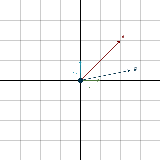
In the standard basis, the geometric vectors in the figure are represented as

\(\mathbf{v} = \begin{bmatrix} 2 \\ 2 \end{bmatrix}, \hspace{0.5cm} \mathbf{w} = \begin{bmatrix} \frac{1}{2} \\ \frac{5}{2} \end{bmatrix}\)

Numerically, this is not the prettiest representation. You might think I’m overemphasizing this point, but there are situations where choosing the wrong basis makes a problem much harder, or even impossible, to solve in practice. So keep this in mind: the choice of basis matters.

From this point on, I will assume you know the difference between geometric vectors and vectors in \(\mathbb{R}^n\). To keep things simple and emphasize the ideas we are focusing on, I will use bold notation (lists of numbers) to represent vectors in the upcoming figures. When you see a geometric vector in a figure, it will be labeled using its numerical representation in the standard basis shown above. I’ll let you know whenever I’m using a different basis. I will also use the word vector exclusively to refer to its numerical representation. When I am explicitly referring to the arrow itself, I will use the term geometric vector.

We can even visualize \(\mathbb{R}^3\) using three basis vectors, each representing a specific direction in space, as shown below.

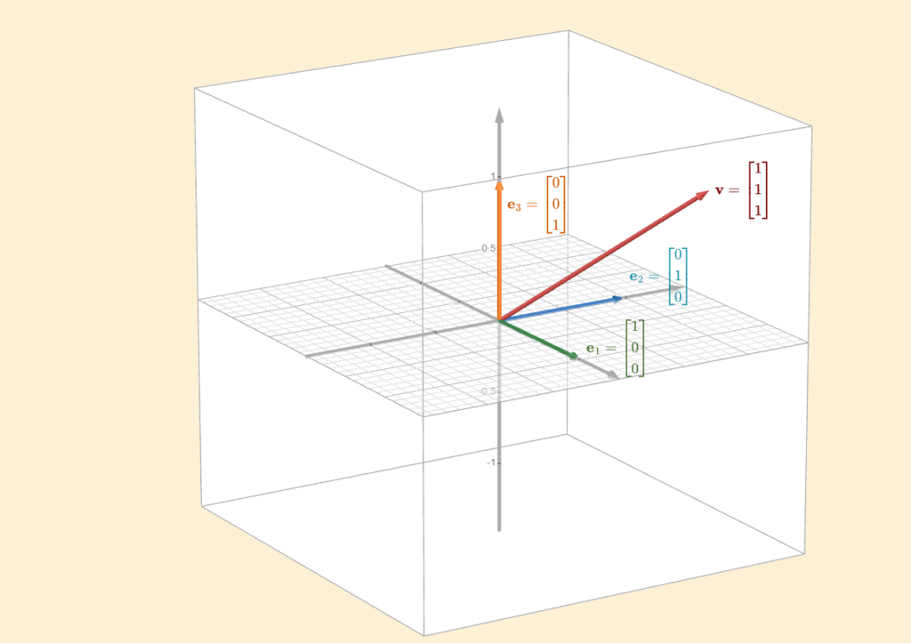
Think of the tip of an arrow as a point in space. Now, imagine all possible points in that space. Each of these points can be described by a list of numbers. If we take all these lists and group them together, we get \(\mathbb{R}^n\).

Earlier, we talked about scaling the basis vectors to get the right representation. But what does scalar multiplication actually look like geometrically?

Scaling Vectors

Multiplying a vector by a scalar changes its size and possibly its direction. If the scalar is greater than \(1\), the vector becomes longer. If it’s between \(0\) and \(1\), the vector shortens. If the scalar is negative, the vector flips direction. We call it a ‘scalar’ because it scales the vector. It’s important to note that while a scalar can stretch, shrink or flip a vector, it can’t rotate it, rotation isn’t possible through scalar multiplication alone.

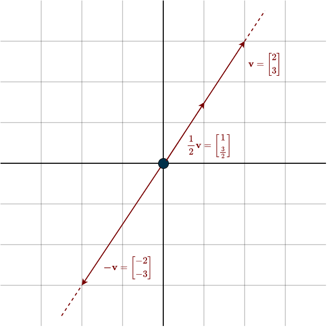
You can see the additive inverse visually here \(\mathbf{v} + (-\mathbf{v}) = \mathbf{0}\). The two vectors cancel each other out, leaving only the zero vector, which is located exactly at the origin. Speaking of which, what does vector addition look like visually?

Vector Addition

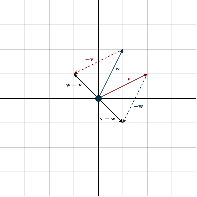
Adding two vectors geometrically is straightforward. This is one of the few cases where you move a vector away from the origin. You simply place the tail of one vector at the head of the other. The order doesn’t matter, the result is the same, because vector addition needs to be commutative.

Subtraction requires a bit more attention. As we saw on the previous page, subtraction is really just addition with additive inverses. However, it’s important to note that \(\mathbf{v}-\mathbf{w}\) and \(\mathbf{w}-\mathbf{v}\) are not the same, since \(\mathbf{-v}\) and \(\mathbf{-w}\) are different. It’s also interesting to point out that the additive inverse of \(\mathbf{v}-\mathbf{w}\) is \(\mathbf{w}-\mathbf{v}\) (since \(-(\mathbf{w}-\mathbf{v}) = -\mathbf{w} + \mathbf{v} = \mathbf{v}-\mathbf{w}\)).

Next, we’ll introduce a new concept that follows directly from the definition of a vector space.

Linear Combination

By adding vectors, we create new vectors, which follows from the closure property of a vector space. This means we can write some vector as a combination of other vectors. Looking at the image above, we can call the resulting sum vector \(\mathbf{x}\) and describe it like this:

\(\mathbf{x} = \mathbf{v} + \mathbf{w}\)

We call such a combination a linear combination. So, \(\mathbf{x}\) is a linear combination of \(\mathbf{v}\) and \(\mathbf{w}\). Now, let’s look at it more generally:

The definition above simply means we take multiples of some vectors and add them together to create a new vector. It’s called a ‘linear’ combination because the scalars are linear. Now, here’s the interesting part: given two vectors, there isn’t just one combination you can create, but infinitely many.

Consider this: Suppose you have a vector \(\mathbf{v}\). When you scale this vector, you can generate any vector that points in the same direction, this forms a line (as shown by the dotted line in the figure below). However, you can’t produce vectors that lie in a different direction using \(\mathbf{v}\) alone.

Now, introduce another vector \(\mathbf{w}\). Like \(\mathbf{v}\), it has its own direction, and by scaling it, you can create any vector along that direction. The key idea is that vector addition lets us combine these two directions.

By adding scaled versions of \(c\mathbf{v}\) and \(d\mathbf{w}\), we can generate an entire plane of vectors through linear combinations. In fact, this allows us to create every possible vector in two-dimensional space. Look at the following figure:

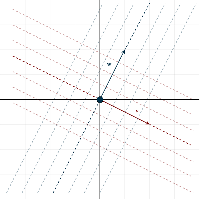
Here, the dotted lines are spaced \(\frac{1}{4}\)​ of the vector apart. So, the dotted line above \(\mathbf{v}\) represents any vector that can be written as the linear combination \(\mathbf{x} = c \cdot \mathbf{v} + \frac{1}{4} \mathbf{w} \). The dotted line along \(\mathbf{v}\) is simply offset by some factor of \(\mathbf{w}\). The same is true for the dotted lines with \(\mathbf{w}\), as they are offset by some factor of \(\mathbf{v}\). The image above illustrates the geometry. In theory, with infinite precision, these closely spaced dotted lines fill the entire plane, allowing us to create every possible vector within that space.

Now, we want to measure how many vectors can be produced as linear combinations of some given vectors.

Span

If we look at the figure from above, it’s easy to see that we can create any vector in 2D space using the vectors \(\mathbf{v}\) and \(\mathbf{w}\). That means the span of \(\mathbf{v}\) and \(\mathbf{w}\) is the entire 2D space, \(\mathbb{R}^2\). If you look at the scaling-vector figure, the span of a single vector consists only of multiples of that vector (the dotted line). So if our vector space were \(\mathbb{R}\) (1D), then one vector would be enough to cover every possible vector in that space. If our vector space were \(\mathbb{R}^2\), then two vectors would be enough to create every vector and span the whole space. For \(\mathbb{R}^3\), we’d need three vectors, and so on, you get the idea.

However, there’s one important detail: this only works if the vectors actually point in different directions. Otherwise, we can’t create new directions or reach the full space. In other words, the vectors need to be linearly independent. But what exactly does that mean?

Linear Independence

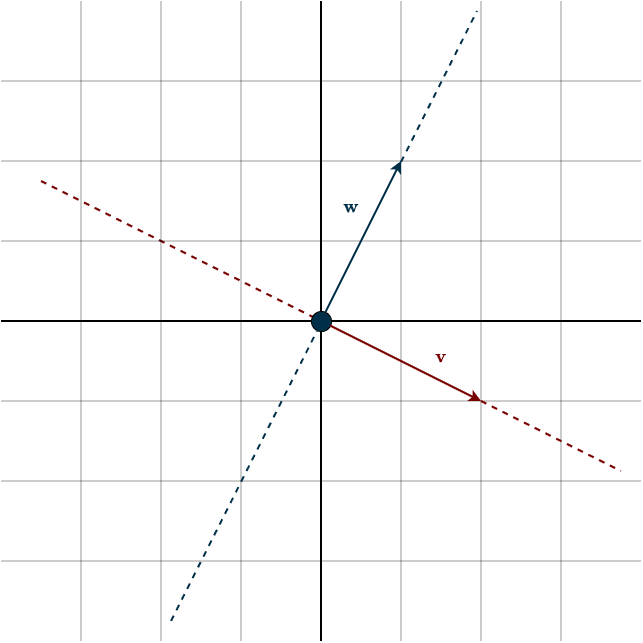
Imagine two vectors pointing in the same direction:

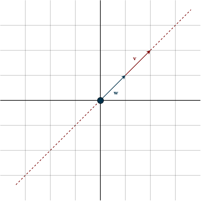
In this case, no matter how we combine the vectors \(\mathbf{v}\) and \(\mathbf{w}\), we remain restricted to the direction they both share. For example, we cannot generate the vector \((-1, -1)\). One vector is simply a scalar multiple of the other: \(\mathbf{w} = \frac{1}{2}\mathbf{v}\) or \(\mathbf{v} = 2\mathbf{w}\). This means we can replace one with a linear combination of the other. Put simply, the second vector does not introduce a new direction or dimension; it’s redundant. It can be replaced without losing any information or dimensionality. We call such vectors linearly dependent. In contrast, vectors that point in different directions, where removing one actually leads to a loss of information or dimension, are called linearly independent.

A single vector is considered linearly independent in \(\mathbb{R}\) if it is non-zero. Two non-zero vectors in \(\mathbb{R^2}\) are linearly independent if they are not scalar multiples of each other, that is, they point in different directions. Three non-zero vectors in \(\mathbb{R^3}\) are linearly independent if the first two are independent and the third is not a linear combination of the previous ones. More generally, a set of non-zero vectors is considered linearly independent if each new vector does not lie in the span of the preceding ones.

(Note that two independent vectors in \(\mathbb{R}^2\) are sufficient to span the entire space. Therefore, any third vector in \(\mathbb{R}^2\) must lie within the span of the first two, meaning that three vectors in \(\mathbb{R}^2\) will always be linearly dependent. We will see this shortly with the definition of the dimension of a vector space.)

The mathematical definition is, as expected, a bit more abstract:

To understand where this definition comes from, consider this:

Suppose you have a list of vectors \(\mathbf{v}_1, \dots, \mathbf{v}_m \in V\) and another vector \(\mathbf{v}\) that lies in the span of the previous vectors, so \(\mathbf{v} \in \text{span}(\mathbf{v}_1, \dots, \mathbf{v}_m)\). By the definition of the span, this means there exists a linear combination of the given vectors that equals:

\(\mathbf{v} = a_1 \cdot \mathbf{v}_1, \dots, a_m \cdot \mathbf{v}_m\)

Now, we want to ask if this combination is unique. Suppose, for instance, there is a second linear combination, say:

\(\mathbf{v} = c_1 \cdot \mathbf{v}_1, \dots, c_m \cdot \mathbf{v}_m\)

If we subtract the two equations, we get:

\(0 = (a_1 – c_1) \cdot \mathbf{v}_1, \dots, (a_m – c_m) \cdot \mathbf{v}_m\)

If the only way to express zero as a linear combination of \(\mathbf{v}_1, \dots, \mathbf{v}_m\) is by setting all the scalars to zero, this implies that \(a_k – c_k = 0\) for all \(k\), which means \(a_k = c_k\)​. Therefore, the linear combination was unique. In other words, if the vectors are linearly independent, then linear combinations of these vectors are unique.

If we look at our example in the figure above, we can find multiple combinations that equal zero: \(-2\mathbf{w} + \mathbf{v} = -4\mathbf{w} + 2\mathbf{v} = \dots = 0\). Not unique, not linearly independent. This definition leads to some important facts to know:

• Every list of vectors in \(V\) containing the \(\mathbf{0}\) vector is linearly dependent. Since you can choose any scalar, multiply it by the zero vector, and zero out every other vector in the combination, the result will be zero.
• If some vectors are removed from a linearly independent list, the remaining list is also linearly independent.

To wrap up this chapter, we will combine the definitions of span and linear independence.

Basis

In a vector space, such as \(\mathbb{R}^2\), we want the basis to uniquely represent every possible vector. If the list of vectors does not span the space, we won’t be able to produce every vector. Similarly, if the vectors are not linearly independent, the linear combination will not be unique. In other words: A list of vectors in a vector space that is small enough to be lineraly independent and big enough so the linear combinations of the list fill up the vector space is called a basis of the vector space.

We made our own basis vectors at the top of this page, but most of the figures so far use the standard ones. We can easily verify that they are linearly independent because they point in different directions (or, equivalently, there is no nonzero linear combination that produces the zero vector). Moreover, they span the entire space, since two linearly independent vectors are sufficient to span \(\mathbb{R}^2\). If we were to add a third vector, it could no longer form a basis, as the set would no longer be independent.

We will be studying the vector space \(\mathbb{R}^n\). This is the tool we’ll use to help solve our machine learning problems. Later, when we translate real-world data into the computer, whether images, company sales data, or housing prices, we will be working explicitly in this vector space. We convert this data into \(\mathbb{R}^n\) using a basis.

Here’s the important point: all bases are created equal, until we define a specific problem. Once the problem is defined, we choose the basis that makes computations easiest. In other words, the problem dictates which basis is most useful. Unfortunately, many people pick bases randomly, or stick with the standard basis, simply because it’s common, even if it’s not the most efficient choice. When all you have is a hammer, everything starts to look like a nail. The standard basis is a very good hammer, but not every problem is a nail.

A vector is an abstract mathematical object. Depending on the basis we choose, it can have different representations, but it’s still the same underlying object. The vector itself doesn’t change, only the coordinates we use to describe it do. Think of it like measuring a box with different tools: a metric ruler, an inch ruler, or even your thumb. The measurements will be different, but the box itself remains the same.

Bases are important to understand, so make sure you’ve got the concept. Switching between different bases will be important later on, but for now, just assume the standard basis, as we’ve done throughout this section (changing between bases can be a bit confusing at first).

Using the definition of a basis, we can now define the dimension of a vector space.

Dimension

For a given vector space \(\mathbb{R}^n\), any two bases have the same number of vectors, specifically, \(n\). For example, every basis of \(\mathbb{R}^2\) contains exactly two vectors, regardless of which basis we choose. This useful fact allows us to define the dimension of a vector space as follows:

Finite dimensional vector space means the following:

If we can construct a list of vectors that spans a vector space, then we say the space is finite-dimensional. (Keep in mind that in our definition, lists always have a finite length.) The vector space \(\mathbb{R}^n\), which is our primary focus, is finite-dimensional because we can always find a list of vectors that spans it. In this course, we will work exclusively with finite-dimensional vector spaces, since our attention is restricted to \(\mathbb{R}^n\). However, it is important to keep in mind that not every concept that holds for finite-dimensional spaces extends to infinite-dimensional ones.

A classic example of an infinite-dimensional vector space is the space of all polynomials. A basis for this space can be written as

\((1, x, ,x^2, x^3, \dots)\)

but this is infinite, its length is unbounded because the degree of a polynomial can always increase.

These definitions lead to several key facts:

• \(\text{dim}(\mathbb{R}^n) = n\) for every positive integer \(n\). For example, the dimension of \(\mathbb{R}^2 = 2\).
• Any linearly independent list of vectors in \(\mathbb{R}^n\) whose length equals \(\text{dim}(\mathbb{R}^n)\) is a basis of \(\mathbb{R}^n\). For instance, in \(\mathbb{R}^2\), any list of two linearly independent vectors automatically forms a basis.

Summary

• Geometric vectors can be represented in \(\mathbb{R}^n\) using a basis, but the vectors in \(\mathbb{R}^n\) are just representations, not the geometric vectors themselves.
• You can form new vectors from a given set of vectors by taking linear combinations of them.
• The collection of all such linear combinations is called the span of those vectors.
• A list of vectors is linearly independent when no vector can be written as a linear combination of the others. Geometrically, they each point in a different direction.
• When a list of vectors both spans the entire vector space and is linearly independent, it is called a basis of that vector space.
• All bases are created equal; the choice depends on the problem at hand.
• The dimension of a vector space is the length of its basis.