Eigenvectors and Eigenvalues

Which vectors do not move under a linear transformation?

Linear transformations move vectors: some are rotated, others are distorted. But there are special vectors that are only stretched or shrunk, their direction remains unchanged. These are called eigenvectors, and the factor by which they are scaled is the eigenvalue. A linear transformation is an abstract mathematical object that can be represented numerically in many different ways. We can move between these representations using a change of basis. Eigenvalues and eigenvectors give us the cleanest and simplest form of a transformation: a diagonal matrix. Transforming a matrix into this form, by switching from the standard basis to one made of its eigenvectors, is called diagonalization. However, not every matrix is diagonalizable. A key exception is symmetric matrices: they are always diagonalizable, have real eigenvalues, and orthogonal eigenvectors. All numerical representations of the same linear transformation are called similar matrices, and they share the same eigenvalues. In practice, eigenvalues and eigenvectors are computed numerically using algorithms such as the QR iteration.

What Are Eigenvectors and Eigenvalues?

Consider the following matrix:

$A = \begin{bmatrix} 1 & 1 \\ 2 & 0\end{bmatrix}$

When we apply it to some vector, you can see that its direction changes. After the linear transformation, the vector points in a different direction than before.

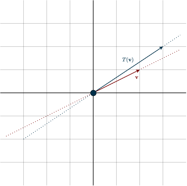
This generally happens to almost every vector, except for some special ones. Look at what happens to these special vectors.

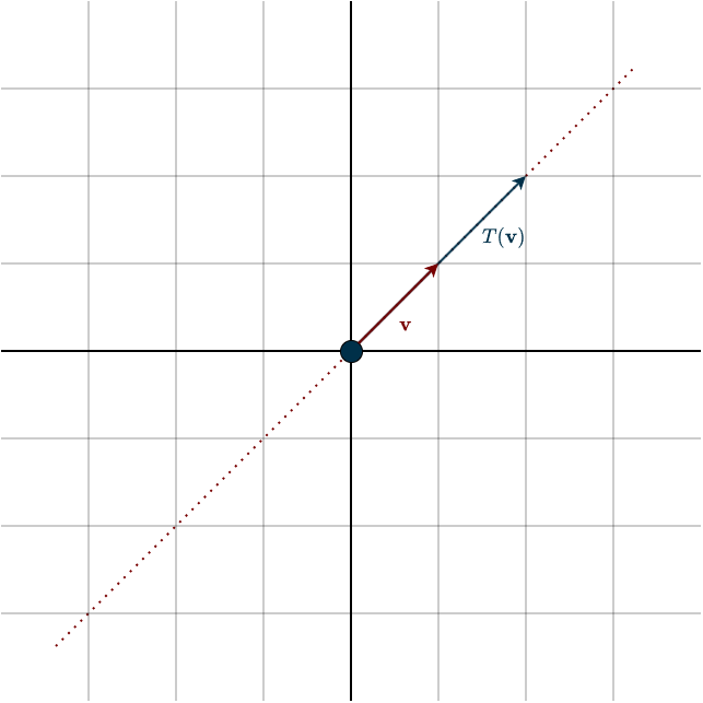
Notice that both vectors share the same direction. One is simply a multiple of the other. This means that this special vector has only been stretched or squished, its direction did not change. We call these special vectors eigenvectors, and the amount by which they are scaled the eigenvalue. In this example, the eigenvalue is $2$. But this is just one example. Eigenvalues can also be negative, complex, or zero. The case where the eigenvalue is zero is particularly interesting. If the eigenvalue represents the scalar that multiplies a vector whose direction does not change under the transformation, then an eigenvalue of zero means that this vector has been completely crushed to the zero vector. In other words, a dimension has been lost, the transformation is singular.

So eigenvalues can tell us quite a lot about a linear transformation, and this information does not depend on the coordinate representation. It relates purely to the transformation itself. Let’s capture this idea formally:

$A\mathbf{v} = \lambda \mathbf{v}$

Here, $\lambda$ is the eigenvalue, the scalar that multiplies the eigenvector $\mathbf{v}$.

Notice something important here. For this equation to make sense, $\mathbf{v}$ and $\lambda \mathbf{v}$ must live in the same vector space. That means the input and output spaces of the transformation must be the same. In other words, we can only talk about eigenvectors and eigenvalues for operators, linear transformations that map a vector space to itself. In matrix terms, this means we are working with square matrices. (Also note that the eigenvector must be nonzero.)

Because of this, we cannot talk about eigenvalues of a rectangular matrix and its corresponding linear transformation. However, there is a closely related concept called the Singular Value Decomposition (SVD), where we work with singular values instead. We will get to that soon.

Focus on the eigenvector in the figure, specifically the dotted line. Remember that this dotted line represents the span of the eigenvector, the set of all vectors that point in the same direction. In simpler terms, it includes all scalar multiples of that eigenvector. Together, these vectors form a subspace.

What’s interesting is that every vector in this subspace is stretched by the same factor, namely $\lambda$. So the transformation scales every vector in this direction by the same amount. This means that each eigenvalue $\lambda$ is associated with a vector space consisting of all vectors that are scaled by that factor. We call this vector space the eigenspace. Formally,

Suppose $T \in \mathcal{L}(V)$ and $\lambda \in F$. The eigenspace of $T$ corresponding to $\lambda$ is the subspace $E(\lambda, T)$ of $V$ defined by

$E(\lambda, T) = \text{null}(T \; – \; \lambda I) = \{\mathbf{v} \in V : T\mathbf{v} = \lambda \mathbf{v}\}$

Hence $E(\lambda, T)$ is the set of all eigenvectors of $T$ corresponding to $\lambda$, along with the $0$ vector.

You might wonder why the eigenspace is defined as the nullspace of $T \; – \; \lambda I$. To see where this comes from, we just need to rewrite the eigenvalue equation. Start with the definition of an eigenvector

$T \mathbf{v} = \lambda \mathbf{v}$

Now move everything to one side

$T \mathbf{v} \; – \; \lambda \mathbf{v} = 0$

Next, rewrite $\lambda \mathbf{v}$ using the identity transformation $I$

$\begin{align} T \mathbf{v} \; – \; \lambda I \mathbf{v} &= 0 \\\\ (T \; – \; \lambda I) \mathbf{v} &= 0 \end{align}$

This shows that eigenvectors are exactly the vectors that are mapped to zero by the transformation $T \; – \; \lambda I$. In other words, they lie in the nullspace of $T \; – \; \lambda I$ The vectors spanning this nullspace are precisely the eigenvectors we are looking for, and each of them is scaled by the corresponding eigenvalue $\lambda$.

Let’s look at some useful properties of eigenvalues.

For triangular matrices, the eigenvalues can be found directly on the diagonal.
Diagonal matrices are a special case of triangular matrices, so their eigenvalues can also be read directly from the diagonal.
If one eigenvalue is zero, then the corresponding linear transformation is singular, and vice versa.
For commuting operators, meaning $TS=ST$, interesting relationships can arise between their eigenvalues and eigenvectors. In many cases, commuting operators share the same eigenvectors. When this happens, the eigenvalues behave nicely: the eigenvalues of $S + T$ are the sums of the corresponding eigenvalues of $S$ and $T$, and the eigenvalues of $ST$ are the products of their corresponding eigenvalues.

Okay, the concept of vectors that don’t change direction under a linear transformation is interesting enough, but why should we care? To start answering this, we need to take a small step back.

Change of Basis

Recall that a basis is what creates our coordinate system and determines how we numerically represent vectors. But a vector itself is an abstract mathematical object, it can have many different numerical representations depending on which basis we choose. This is similar to measuring a box using different units. The numbers change, but the box itself remains the same. Because of this, the same vector can have different coordinate representations, depending on the coordinate system being used. This naturally leads to a question: If two people use different bases, is there a way to translate between their coordinate systems?

Let’s make this situation concrete. Suppose you are using the standard basis, the one we have used throughout most of this course. However, your friend prefers a different basis because he thinks it makes him look cooler and more unique. He uses the following basis vectors:

$\mathbf{b}_1 = \begin{bmatrix} 1 \\ 1 \end{bmatrix}, \hspace{1cm} \mathbf{b}_2 = \begin{bmatrix} 1 \\ -1 \end{bmatrix}$

Notice something important: these coordinates are written in the standard basis. In other words, these are your friend’s basis vectors, just expressed in our language. In your friend’s own coordinate system, these vectors would simply look like the standard basis vectors do to us: $(1,0)$ and $(0,1)$.

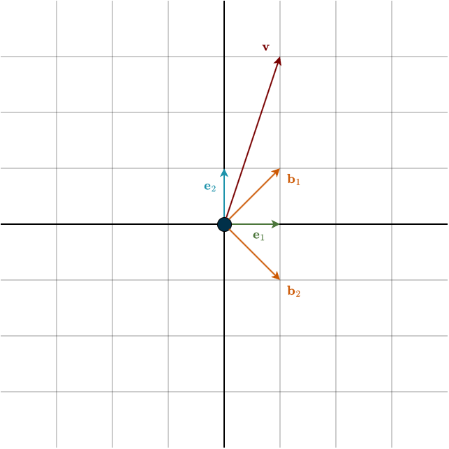
Now consider the vector $\mathbf{v}$ from the figure. Depending on the basis we use, it can have two different representations:

$\mathbf{v} = \begin{bmatrix} 1 \\ 3 \end{bmatrix}, \hspace{1cm} [\mathbf{v}]_{\mathcal{B}} = \begin{bmatrix} 2 \\ -1 \end{bmatrix}$

The notation $[\mathbf{v}]_{\mathcal{b}}$ means that the coordinates are given relative to your friend’s basis $\mathcal{B}$. If you were to give your friend the vector $1, 3$, he would assume those numbers refer to his coordinate system, not yours. As a result, he would end up with a completely different vector. So even though you are talking about the same vector, the two of you are speaking different coordinate languages. You are speaking English, and he is speaking Spanish. We therefore need a way to translate between the two coordinate systems. How do we do that?

Simple, recall that every vector can be written as a linear combination of its basis vectors. In your friend’s coordinate system,

$[\mathbf{v}]_{\mathcal{B}} = v_1 \cdot \mathbf{b}_1 + v_2 \cdot \mathbf{b}_2$

Now we express those basis vectors in the standard coordinate system

$\mathbf{v} = v_1 \cdot \begin{bmatrix} 1 \\ 1 \end{bmatrix} + v_2 \cdot \begin{bmatrix} 1 \\ -1 \end{bmatrix}$

This gives us exactly the translation we need. The scalars $v_1$ and $v_2$ refer to your friend’s basis vectors. But if we express those basis vectors in our coordinate system, then any linear combination of them automatically produces a vector in our coordinates. For example, suppose your friend sends you the vector

$[\mathbf{v}]_{\mathcal{B}} = \begin{bmatrix} 2 \\ -1 \end{bmatrix}$

This means that in the standard basis the vector is

$\mathbf{v} = 2 \cdot \begin{bmatrix} 1 \\ 1 \end{bmatrix} + (- 1) \cdot \begin{bmatrix} 1 \\ -1 \end{bmatrix} = \begin{bmatrix} 2 \\ 2 \end{bmatrix} + \begin{bmatrix} -1 \\ 1 \end{bmatrix} = \begin{bmatrix} 1 \\ 3 \end{bmatrix}$

Remember that a linear combination like this can be written as a matrix–vector product.

$\mathbf{v} = B [\mathbf{v}]_{\mathcal{B}} = \begin{bmatrix} 1 & 1 \\ 1 & -1 \end{bmatrix} [\mathbf{v}]_{\mathcal{B}}$

The matrix $B$ is called the change of basis matrix because it converts coordinates from your friend’s basis into the standard basis. To go the other direction, we simply invert the matrix

$[\mathbf{v}]_{\mathcal{B}} = B^{-1} \mathbf{v} = \begin{bmatrix} \frac{1}{2} & \frac{1}{2} \\ \frac{1}{2} & -\frac{1}{2}\end{bmatrix} \begin{bmatrix} 1 \\ 3 \end{bmatrix} = \begin{bmatrix} 2 \\ -1\end{bmatrix}$

Notice that this matrix must be invertible. The reason is that its columns form a basis, and by definition a basis must consist of linearly independent vectors. It shouldn’t be surprising that this also only works for operators, that is, square matrices. Losing information would make the translation much more difficult.

Vectors are not the only objects represented using coordinates and a basis. Linear transformations are too. A linear transformation itself does not change, but its matrix representation depends on the basis we choose. Suppose then, that you have created a transformation $T$ that you are very proud of and want to show your friend. In the standard basis it is represented by the matrix

$A = \begin{bmatrix} 0 & -1 \\ 1 & 0 \end{bmatrix}$

This matrix represents a 90° counterclockwise rotation.

If you naively send this matrix to your friend and he applies it to his coordinate vector, he gets

$A [\mathbf{v}]_{\mathcal{B}} = \begin{bmatrix} 0 & -1 \\ 1 & 0 \end{bmatrix} \begin{bmatrix} 2 \\ -1 \end{bmatrix} = \begin{bmatrix} 1 \\ 2 \end{bmatrix}_{\mathcal{B}}$

These coordinates correspond to some vector in the upper-right quadrant, which is clearly not the correct rotated vector. Why did this happen? Because the matrix $A$ expects vectors expressed in the standard basis. Feeding it vectors expressed in a different basis produces meaningless results.

Think of matrices as machines that expect a specific type of input. Our matrix $A$ expects vectors written in the standard basis. If we give it vectors expressed in your friend’s basis, it does not know how to interpret them. But we already know how to translate between the bases.

So we simply:

Translate your friend’s vector into the standard basis
Apply the transformation
Translate the result back

The combined matrix $M$ that performs these steps is

$M = B^{-1}AB$

To go the other way, we simply rewrite the equation as

$A = BMB^{-1}$

Now, applying the matrix $M$ to your friend’s coordinates gives

$T([\mathbf{v}]_{\mathcal{B}}) = B^{-1}AB [\mathbf{v}]_{\mathcal{B}} = \begin{bmatrix} \frac{1}{2} & \frac{1}{2} \\ \frac{1}{2} & -\frac{1}{2}\end{bmatrix} \begin{bmatrix} 0 & -1 \\ 1 & 0 \end{bmatrix} \begin{bmatrix} 1 & 1 \\ 1 & -1 \end{bmatrix} \begin{bmatrix} 2 \\ -1 \end{bmatrix} = \begin{bmatrix} -1 \\ -2 \end{bmatrix}$

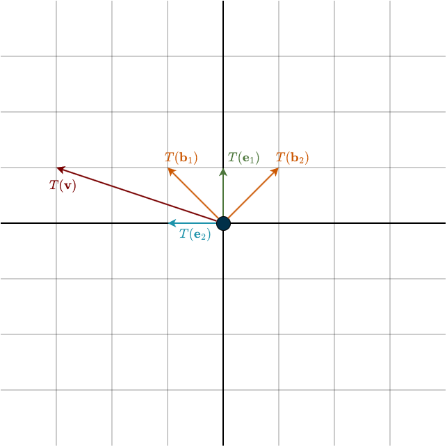
When checking this calculation yourself, remember that the intermediate results are expressed relative to the standard basis vectors $\mathbf{e}_1, \mathbf{e}_2$, not the transformed vectors $T(\mathbf{e}_1), T(\mathbf{e}_2)$. The same is true for the result. The final coordinates refer to the original basis vectors $\mathbf{b}_1$ and $\mathbf{b}_2$, not the transformed vectors $T(\mathbf{b}_1)$ and $T(\mathbf{b}_2)$. If this feels confusing, take another look at the first figure of this section.

Okay, how does this relate to eigenvectors and eigenbasis?

Diagonalization

If linear transformations can be expressed in any coordinate system we choose, a natural question arises: which coordinate system is the best? Or rather, which one is the simplest?

Which representation makes our work easiest and simplifies calculations the most? If I asked you: Which matrix is the simplest? The easiest to work with? What would you answer?

Take a look at diagonal matrices. Diagonal matrices are a special case of triangular matrices where all entries are zero except those on the main diagonal. Consider the example

$D = \begin{bmatrix} 2 & 0 & 0 \\ 0 & 5 & 0 \\ 0 & 0 & 7 \end{bmatrix}$

What does this matrix actually do? It only scales the basis vectors. If we multiply this matrix by some vector, each coordinate direction is scaled by the corresponding diagonal entry

$D \mathbf{v} = \begin{bmatrix} 2 & 0 & 0 \\ 0 & 5 & 0 \\ 0 & 0 & 7 \end{bmatrix} \begin{bmatrix} v_1 \\ v_2 \\ v_3 \end{bmatrix} = \begin{bmatrix} 2 \cdot v_1 \\ 5 \cdot v_2 \\ 7 \cdot v_3 \end{bmatrix}$

There is no rotation, no skewing, no strange distortion, just stretching along the coordinate axes. The matrix is simply saying:

make the first direction $2$ times larger
make the second direction $5$ times larger
make the third direction $7$ times larger

Nothing more.

Now think about what kind of vectors behave like this. We are talking about vectors that only get scaled and do not change direction. Does that sound familiar? That is exactly what happens to eigenvectors. So there must be a connection here. There must be some way to use eigenvectors to transform a matrix $A$ into a diagonal matrix.

Recall the definition of an eigenvector

$A\mathbf{v} = \lambda \mathbf{v}$

However, this equation only describes one eigenvector. Suppose then that the matrix $A$ has $n$ eigenvectors

$\mathbf{v}_1, \mathbf{v}_2, \dots, \mathbf{v}_n$

with corresponding eigenvalues

$\lambda_1, \lambda_2, \dots, \lambda_n$

Each eigenvector satisfies its own equation

$A\mathbf{v}_1 = \lambda_1 \mathbf{v}_1$

$A\mathbf{v}_2 = \lambda_2 \mathbf{v}_2$

$\vdots$

$A\mathbf{v}_n = \lambda_n \mathbf{v}_n$

So instead of a single equation, we actually have a whole system of equations. We can organize this system neatly by placing all eigenvectors into a matrix $X$, where each column is an eigenvector

$X = \begin{bmatrix} | & | & & | \\ \mathbf{v}_1 & \mathbf{v}_2 & \dots & \mathbf{v}_n \\ | & | & & |\end{bmatrix}$

Now consider the matrix product $AX$. Remember that in Case 2 matrix multiplication from the matrices chapter, we can think of the product as Matrix $A$ multiplying each column of Matrix $X$. In other words, the result comes from applying Matrix $A$ to every column of $X$. This gives us the left-hand side of the equation

$AX = \begin{bmatrix} A\mathbf{v}_1 & A\mathbf{v}_2 & \dots & A\mathbf{v}_n \end{bmatrix}$

Using the same eigenvector matrix $X$, we can obtain the right-hand side of the equation by introducing a diagonal matrix $\Lambda$, where each diagonal entry is an eigenvalue corresponding to its respective eigenvector.

$\Lambda = \begin{bmatrix} \lambda_1 & 0 & \dots & 0 \\ 0 & \lambda_2 & \dots & 0 \\ \vdots & & \ddots & \vdots \\ 0 & 0 & \dots & \lambda_n \end{bmatrix}$

Consider $X \Lambda$. Using the same matrix multiplication idea as above, we get

$X\Lambda = \begin{bmatrix} \lambda_1 \mathbf{v}_1 & \lambda_2 \mathbf{v}_2 & \dots & \lambda_n \mathbf{v}_n \end{bmatrix}$

Now that we have both sides of the equation (and since we can substitute $A \mathbf{v}_i$ with $\lambda_i \mathbf{v}_i$), we can write the entire eigenvector system in a more compact form

$AX = \begin{bmatrix} A\mathbf{v}_1 & A\mathbf{v}_2 & \dots & A\mathbf{v}_n \end{bmatrix} = \begin{bmatrix} \lambda_1 \mathbf{v}_1 & \lambda_2 \mathbf{v}_2 & \dots & \lambda_n \mathbf{v}_n \end{bmatrix} = X\Lambda$

$AX = X\Lambda$

We can rearrange this equation to obtain

$\Lambda = X^{-1}AX$

Notice what happened here. We transformed the matrix $A$ into the diagonal matrix $\Lambda$. This process is called diagonalization. However, there is an important requirement: the matrix $X$ must be invertible. This means the eigenvectors must be linearly independent. If they are not independent, $X^{−1}$ does not exist and the diagonalization fails. Now, look carefully at the expression

$X^{-1}AX$

Does it look familiar? It should, it is exactly the same structure as a change of basis. What we are doing is expressing the linear transformation represented by $A$ in a different coordinate system. But this time, the new basis is formed by the eigenvectors of $A$. We call this basis the eigenbasis. And in this coordinate system, the transformation becomes incredibly simple: it is represented by the diagonal matrix $\Lambda$. In other words, diagonalization gives us the cleanest and simplest possible representation of the transformation.

To see why this is useful in practice, we can rewrite the expression above in another form

$A = X \Lambda X^{-1}$

Now imagine you want to compute powers of $A$, meaning you apply the linear transformation many times in succession. If you tried to do this directly with the matrix $A$, it would quickly become tedious. Even for a computer, matrix multiplication is relatively expensive. But things become much simpler once we work with eigenvectors. Consider what happens when we square $A$

$A^2 = AA = X \Lambda X^{-1}X \Lambda X^{-1} = X \Lambda^2 X^{-1}$

More generally, for any power $k$,

$A^k = X \Lambda^k X^{-1}$

So taking powers of $A$ reduces to taking powers of the diagonal matrix $\Lambda$. And powers of a diagonal matrix are easy to compute, you simply raise each diagonal entry to that power

$\Lambda^k = \begin{bmatrix} \lambda_1^k & 0 & \dots & 0 \\ 0 & \lambda_2^k & \dots & 0 \\ \vdots & & \ddots & \vdots \\ 0 & 0 & \dots & \lambda_n^k \end{bmatrix}$

This also tells us something interesting: $A^k$ has the same eigenvectors as $A$, and only the eigenvalues change, from $\lambda$ to $\lambda^k$. Intuitively, this makes sense. Eigenvectors are precisely the directions that a matrix does not rotate or change. The matrix $A$ only stretches or compresses them. So no matter how many times we apply $A$, those directions remain fixed. However, every time we apply $A$, the eigenvectors are scaled by their corresponding eigenvalue. If we apply $A$ twice, the scaling happens twice. Apply it $k$ times, and the scaling becomes $\lambda^k$.

You can think of this as the difference between static and dynamic problems in linear algebra. Gaussian elimination was useful for static problems. We encountered a system of linear equations, translated it into matrix form $A\mathbf{x} = \mathbf{b}$, and then solved for $\mathbf{x}$ exactly (or found the closest possible solution).

Eigenvectors and eigenvalues, on the other hand, help us understand dynamic systems, situations where something evolves over time. In these cases, the state of the system changes according to

$\mathbf{x}_{t+1} = A\mathbf{x}_t$

Here the matrix $A$ is applied repeatedly, which means we are effectively computing powers of $A$. Thanks to diagonalization, we can do this efficiently, without making your computer explode.

This idea appears in many real-world applications. For example:

Population models, where we study how populations evolve over time.
Markov chains, where we track how probabilities change step by step.
etc.

When Is a Matrix Diagonalizable?

Diagonalizing a matrix $A$ can be very useful, as we have just seen. However, not every matrix can be diagonalized. First, we need an operator, that is, a square matrix. We cannot talk about eigenvalues and eigenvectors of a rectangular matrix. These concepts only make sense for linear transformations from a vector space to itself. Second, we required that the eigenvector matrix $X$ be invertible. Recall that a matrix is invertible only if its columns form a basis, which means the columns must be linearly independent.

So the key question becomes: When are the eigenvectors linearly independent?

A very important result answers this.

Suppose $T \in \mathcal{L}(V)$. Then every list of eigenvectors of $T$ corresponding to distinct eigenvalues of $T$ is linearly independent.

In other words, distinct eigenvalues guarantee independent eigenvectors. But things become more interesting when eigenvalues are repeated. In that case, we might not get enough eigenvectors.

Example

Consider the matrix

$A = \begin{bmatrix} 3 & 1 \\ 0 & 3 \end{bmatrix}$

For triangular matrices, we can read the eigenvalues directly from the diagonal. So here we see that the eigenvalue $3$ appears twice. In other words, the eigenvalue is repeated. If we compute the eigenvectors (just trust me on this for now, we will see how to calculate them soon), we obtain only one

$\mathbf{v} = \begin{bmatrix} 1 \\ 0 \end{bmatrix}$

Of course, any scalar multiple of this vector is also an eigenvector. But essentially, we only have one independent eigenvector. So what happened here? Why do we only get one?

The transformation represented by this matrix stretches space, but it also skews it. This skewing is what destroys the other eigenvector. Remember that skewing simply means tilting vectors in some direction. When vectors tilt, their direction changes. But an eigenvector is a vector whose direction does not change under the transformation. Because the skewing tilts almost every vector, only one direction survives as an eigenvector.

You might wonder: If we have two eigenvalues, which vector does the second one scale?

The key idea is that eigenvalues correspond to eigenspaces, not individual vectors. When eigenvalues are distinct, they correspond to different eigenspaces, which automatically gives us independent eigenvectors. But when eigenvalues are repeated, they can correspond to the same eigenspace.

So if the eigenvalues are the same, does that mean we only get one eigenvector and therefore can’t form $X$?

No, not generally. Repeated eigenvalues can lead to too few eigenvectors, but they do not have to. Consider the matrix

$A = \begin{bmatrix} 3 & 0 \\ 0 & 3 \end{bmatrix}$

This matrix also has the repeated eigenvalue $3$. But this time the matrix is already diagonal. This transformation simply stretches every direction by $3$. Since nothing is skewed or rotated, every vector keeps its direction. That means every vector is an eigenvector. Again, both eigenvalues correspond to the same eigenspace. Notice, however, that this eigenspace has dimension $2$: since our vector space is $\mathbb{R}^2$ and every vector in it is an eigenvector. We just need to choose two linearly independent vectors from it to form our matrix $X$.

To understand this more systematically, we introduce two important numbers.

First, the algebraic multiplicity (AM) of an eigenvalue. This is simply the number of times the eigenvalue appears. For example, if

$\lambda_1 = \lambda_2 = \lambda_3 = 8$

then the eigenvalue $8$ has AM = $3$.

Second, we have the geometric multiplicity (GM). This counts how many linearly independent eigenvectors belong to an eigenvalue. In other words, it is the dimension of the eigenspace associated with that eigenvalue. As we saw earlier, this number depends on the matrix itself. If a matrix does not have enough independent eigenvectors, we call it defective (kind of a rude name).

In general, the following relationship always holds

$GM \leq AM$

If for at least one eigenvalue we have

$GM < AM$

then the matrix is defective. In that case, we do not have enough eigenvectors to span the vector space, and diagonalization is impossible. Note that geometric multiplicity depends on the specific eigenvalue, since different eigenvalues may have different eigenspaces.

Symmetric Matrices and the Spectral Theorem

We’ve just seen that not every square matrix is diagonalizable. But for symmetric matrices, those that represent self-adjoint transformations, something special happens.

The eigenvector matrix becomes orthogonal.
The eigenvectors of a symmetric matrix are orthogonal to each other. If we normalize them to have unit length, they become orthonormal. This gives us the decomposition

$S = Q \Lambda Q^{\top}$

where we use $Q$ instead of $X$ to emphasize that it is an orthogonal matrix. From this decomposition, it’s also easy to see that $S=S^{\top}$.

The eigenvalues are real.
In general, eigenvalues can be real, complex, or zero. But for symmetric matrices, they are always real. This tells us something important about their behavior. Complex eigenvalues usually arise when a transformation involves rotation (or reflections), since rotation changes the direction of every vector, no real vector remains aligned with itself and qualifies as an eigenvector. In the complex setting, rotations can still be interpreted as scaling, which is why complex eigenvalues appear there. Geometrically, this means a symmetric matrix does something quite simple: it rotates the coordinate system ($Q^{\top}$) to align with the eigenvector directions, then applies pure scaling according to the values in $\Lambda$, and finally rotates back ($Q$).

The remarkable part is that all of this holds for every symmetric matrix. This result is known as the spectral theorem. It means we don’t have to worry about special conditions for diagonalizability, symmetric matrices are guaranteed to be diagonalizable.

Similiar Matrices

We know that a linear transformation can look different depending on the basis, and therefore the coordinate system, we choose. Even though the matrix representation changes, the underlying linear transformation remains the same. Because of this, a single linear transformation can have many different matrix representations. All of these matrices are called similar matrices. They represent the same transformation, just expressed in different bases.

So the key idea behind similar matrices is change of basis

$A = X \Lambda X^{-1}$

If we keep $\Lambda$ fixed and change $X$ to another invertible matrix, we obtain a different matrix that is similar to $A$. In other words, we get a different representation of the same linear transformation. This produces an entire family of similar matrices. We can write this idea in a more general form that does not explicitly involve eigenvectors or eigenvalues

$A = BKB^{-1}$

Here:

$B$ is a change-of-basis matrix
$K$ is the matrix representing the same linear transformation expressed in a different basis

One interesting property of similar matrices is that they always have the same eigenvalues. Why is that?

Let $K$ represent the same linear transformation as $A$, but written in a new basis

$K = B^{-1}AB$

Now recall the eigenvector equation

$A \mathbf{v} = \lambda \mathbf{v}$

Since we are changing the basis, the eigenvector $\mathbf{v}$ expressed in the new basis becomes a new coordinate vector $\mathbf{w}$

$ \mathbf{w} = B^{-1}\mathbf{v} \hspace{0.5cm} \Longrightarrow \hspace{0.5cm} \mathbf{v} = B \mathbf{w}$

Now substitute this expression for $\mathbf{v}$ into the eigenvector equation

$A (B \mathbf{w}) = \lambda (B \mathbf{w})$

Next, multiply both sides by $B^{−1}$ to eliminate $B$ on the right-hand side of the equation

$ \begin{align} B^{-1} (A B \mathbf{w}) &= B^{-1} (\lambda B \mathbf{w}) \\\\ (B^{-1} A B) \mathbf{w} &= \lambda B^{-1}B \mathbf{w} \\\\ (B^{-1} A B) \mathbf{w} &= \lambda \mathbf{w}\end{align}$

But $B^{−1}AB=K$, so we obtain

$K \mathbf{w} = \lambda \mathbf{w}$

Notice that the eigenvalue $\lambda$ did not change. Therefore, $A$ and $K$ must have the same eigenvalues. Every eigenvalue of $A$ corresponds to an eigenvalue of $K$, and vice versa. This makes intuitive sense because both matrices describe the same underlying linear transformation. Does this mean the eigenvectors are the same as well? Not quite. They represent the same geometric direction, but their coordinate representations change because we switched bases. Recall the relationship between $\mathbf{v}$ and $\mathbf{w}$

$\mathbf{w} = B^{-1}\mathbf{v}$

So we did not change the geometric vector itself, we only changed how we describe it in coordinates.

How Do We Actually Calculate the Eigenvectors and Eigenvalues?

So far, I’ve only told you what eigenvalues and eigenvectors are. Now it’s time to actually compute them. The traditional “university course” approach is to solve something called the characteristic polynomial. Its roots, that is, the values where the polynomial evaluates to zero, are the eigenvalues. Once you have those, you solve for the nullspace of $A \; − \; \lambda I$ for each eigenvalue to get the corresponding eigenvectors. This method gives you exact results, and it’s perfectly valid… for small matrices. Solving a $2 \times 2$ or $3 \times 3$ system is nice and manageable. But unless you’re working on some todler project, real-world matrices, especially in machine learning, can have thousands of entries. On top of that, there’s no general formula for solving polynomials of degree 5 or higher, and working with polynomials in the first place quickly becomes messy.

So instead, let’s take a more practical route: a numerical approach. Rather than solving a huge polynomial, we’ll approximate the eigenvectors and eigenvalues.

Assume $A$ is diagonalizable. Then any vector can be written as a combination of its eigenvectors

$\mathbf{x}_0 = c_1\mathbf{v}_1 + c_2\mathbf{v}_2 + \dots + c_n\mathbf{v}_n$

We also know that applying $A$ simply scales each eigenvector by its eigenvalue

$\begin{align} A\mathbf{x}_0 &= c_1A\mathbf{v}_1 + c_2A\mathbf{v}_2 + \dots + c_nA\mathbf{v}_n \\\\ &= c_1 \lambda_1 \mathbf{v}_1 + c_2 \lambda_2 \mathbf{v}_2 + \dots + c_n \lambda_n \mathbf{v}_n \end{align}$

If we apply $A$ repeatedly, we get

$\mathbf{x}^k = A^k \mathbf{x}_0 = c_1 \lambda^k_1 \mathbf{v}_1 + c_2 \lambda^k_2 \mathbf{v}_2 + \dots + c_n \lambda^k_n \mathbf{v}_n$

Now here’s where things get interesting. Suppose the eigenvalues are ordered such that

$|\lambda_1| > |\lambda_2| \geq |\lambda_3| \dots$

That is, $\lambda_1$ is strictly the largest in magnitude. If we factor out $\lambda_1^k$, we get

$$\mathbf{x}_k = \lambda_1^k \Big(c_1\mathbf{v}_1 + c_2 \Big(\frac{\lambda_2}{\lambda_1}\Big)^k \mathbf{v}_2 + \dots + c_n \Big(\frac{\lambda_n}{\lambda_1}\Big)^k \mathbf{v}_n \Big)$$

Now notice: since

$$\frac{\lambda_i}{\lambda_1} < 1 $$

raising it to higher powers pushes it toward zero (because $\lambda_1$ is the biggest eigenvalue)

$$\lim_{k \to \infty} \Big(\frac{\lambda_i}{\lambda_1}\Big)^k = 0$$

So as $k$ grows, all terms except the first vanish. What’s left is

$\mathbf{x}_k \approx \lambda^k c_1 \mathbf{v}_1$

In other words, $\mathbf{x}_k$ becomes a multiple of the dominant eigenvector $\mathbf{v}_1$. In practice, we normalize $\mathbf{x}_k$ at each step. This doesn’t change its direction, but it keeps the numbers from blowing up. Geometrically, you can think of this as repeatedly “pushing” the space in a way that gradually aligns everything with the dominant eigenvector. Eventually, everything collapses onto that direction. Now that we have the eigenvector, how do we get the eigenvalue?

Simple. Start with the eigenvalue equation

$A\mathbf{v} = \lambda \mathbf{v}$

You might be tempted to divide by $\mathbf{v}$, but recall from Chapter 1 that this operation is not defined: vector division doesn’t exist. In a vector space, we can add (or substract) vectors and scale them, but not divide them. Instead, we turn that pesky vector into a scalar using the dot product. Multiply both sides by $\mathbf{v}^{\top}$

$\mathbf{v}^{\top} (A \mathbf{v}) = \mathbf{v}^{\top} (\lambda \mathbf{v})$

Since $\lambda$ is a scalar, we can pull it out

$$\begin{align} \lambda \mathbf{v}^{\top} \mathbf{v} &= \mathbf{v}^{\top} (A \mathbf{v}) \\\\ \lambda &= \frac{\mathbf{v}^{\top} (A \mathbf{v})} {\mathbf{v}^{\top} \mathbf{v}}\end{align}$$

This expression is called the Rayleigh quotient. Applying it to our approximation, gives us

$$\lambda_1 \approx \frac{\mathbf{x}_k (A \mathbf{x}_k)}{\mathbf{x}^{\top}_k \mathbf{x}_k}$$

This whole process, starting with a random vector, repeatedly applying $A$, normalizing, and extracting the eigenvalue, is called Power Iteration. It’s simple, but not very efficient. If the largest eigenvalue is close to the second one, it can take a long time before the difference really shows. In addition, there’s a catch: it only gives us the largest eigenvalue and its corresponding eigenvector. Everything else gets washed out in the process. So the natural question is: Wouldn’t it be nice to get all eigenvectors, and all eigenvalues, not just the dominant one?

How about we don’t start with just a single vector, but with $n$ vectors? The only requirement is that $A$ is square. Now, if we naively apply power iteration to this matrix, something familiar happens: all columns end up aligning with the dominant eigenvector. So we’re back to the same issue as before. What we need is a way to stop every column from collapsing into that same dominant direction.

So here’s the idea: at every step, we orthogonalize the matrix.

I explained the QR algorithm using Householder reflections in the last chapter, but for intuition, Gram–Schmidt is easier to think about. Gram–Schmidt takes a basis and makes it orthonormal. You keep the first vector, just normalize it to length one. Then you take the second vector, project it onto the first, and subtract that projection. What’s left is perpendicular to the first vector (look at the figures in the projections chapter, the vector $\mathbf{e}$ is exactly that difference). Then you normalize it. For the third vector, you remove the components in the directions of the first two, and so on. You get the pattern.

Now back to our problem: everything wants to move toward the dominant eigenvector. But with QR, we can actively remove that fastest-growing component. What remains is the second fastest-growing direction. If we remove the first two dominant components, we isolate the third, and so on.

So imagine doing power iteration, but after every step, we orthogonalize the matrix. The second column still tries to align with the dominant eigenvector, but we keep forcing it away. We remove the dominant growth direction, so the next one takes over. In simple terms: let everything grow, then remove the largest part. What’s left reveals the next most dominant direction.

At this point, you might wonder: why would the eigenvalues and eigenvectors stay the same through all of this?

Let me explain. Look at the QR decomposition again

$A = QR$

Rearranging gives

$R = Q^{\top}A$

Now multiply by $Q$ on the right

$RQ = Q^{\top}AQ$

This shows that $RQ$ is related to $A$ by an orthogonal similarity transformation. And as we discussed before, similarity transformations just mean we’re expressing the same linear transformation in a different basis, so the eigenvalues stay the same.

Now let’s see how this works step by step. Start with

$A_0 = A$

Compute the QR decomposition

$A_0 = Q_0 R_0$

Then form a new matrix

$A_1 = R_0Q_0$

Repeat the process. In general, at step $k$

$\begin{align} A_k &= Q_k R_k \\\\ A_{k+1} &= R_k Q_k \end{align}$

Since

$R_k = Q^{\top}_k A_k$

we can write

$A_{k+1} = Q_k^{\top} A_k Q_k$

So every step is a similarity transformation. Now you might ask: okay, we keep changing the basis, how does that give us the eigenvalues?

This is where things get interesting. There’s a fundamental result in linear algebra called Schur decomposition. It tells us that any square matrix can be written as

$A = QTQ^{\top} \hspace{0.5cm} \Longrightarrow \hspace{0.5cm} T = Q^{\top}AQ$

Here $T$ is (quasi-)upper triangular (please note that this should not be confused with the $T$ used to denote the abstract mathematical linear transformation) and $Q$ is orthogonal. In other words, every matrix is similar to an upper triangular one. If we’re working over the complex numbers, $T$ is fully upper triangular. Over the real numbers, we may get small $2×2$ blocks along the diagonal, these correspond to complex conjugate eigenvalue pairs (Don’t worry if you’re not sure what that means, it’s not important right now anyway. Just assume we’re working with real eigenvalues.). That’s why we call it quasi-triangular. Here is an example

$T = \begin{bmatrix} \lambda_1 & * & * & * & * \\ 0 & \lambda_2 & * & * & * \\ 0 & 0 & 2 & 5 & * \\ 0 & 0 & -5 & 2 & * \\ 0 & 0 & 0 & 0 & \lambda_5 \end{bmatrix}$

If all eigenvalues are real, then $T$ is just upper triangular. Why does this matter? Because for triangular matrices, the eigenvalues sit right on the diagonal. And here’s the really fascinating part: if we repeat the QR iteration enough times, the matrix $A_k$ actually converges to this triangular form. In other words, for large $k$,

$A_k \hspace{0.5cm} \longrightarrow \hspace{0.5cm} T$

Each step brings us closer. So by repeatedly applying QR decomposition, we’re not just changing the matrix, we’re gradually revealing its eigenvalues directly on the diagonal. Okay, so we’ve got the eigenvalues, what about the eigenvectors?

Recall the eigenvector equation from earlier. To find the eigenvectors, we compute the nullspace of

$(T \; – \; \lambda_i I)\mathbf{v}_i = \mathbf{0}$

for each eigenvalue $\lambda_i$. This gives us a system of linear equations, and since $T$ is upper triangular, we can solve it efficiently using backward substitution

$\begin{bmatrix} 1 \; – \; \lambda_i & 2 & 3 \\ 0 & 4 \; – \; \lambda_i & 5 \\ 0 & 0 & 6 \; – \; \lambda_i\end{bmatrix} \begin{bmatrix} v_1 \\ v_2 \\ v_3 \end{bmatrix} = \begin{bmatrix} 0 \\ 0 \\ 0\end{bmatrix}$

Be careful here, this is not the same backward substitution we used in the LU chapter. Notice what’s happening above: once we subtract a value $\lambda_i$ from the diagonal entries, at least one diagonal element becomes zero. If there are repeated eigenvalues, there may be more than one. In such cases, our usual backward substitution breaks down. To see why, consider

$\begin{bmatrix} 1 \; – \; \lambda_3 & 2 & 3 \\ 0 & 4 \; – \; \lambda_3 & 5 \\ 0 & 0 & 0\end{bmatrix} \begin{bmatrix} v_1 \\ v_2 \\ v_3 \end{bmatrix} = \begin{bmatrix} 0 \\ 0 \\ 0\end{bmatrix}$

Assume the eigenvalues are distinct and we are working with the third one. Then the last row becomes a zero row. If we now apply backward substitution naively, as before, we run into trouble: the last equation gives $v_3=0$, and since the right-hand side is also zero, this forces $v_2=0$, then $v_1=0$, and so on. In the end, we get the zero vector, which cannot be an eigenvector by definition. So what went wrong? Look at the last equation:

$0 \cdot v_3 = 0$

This equation doesn’t actually constrain $v_3$ at all. It can be anything, because multiplying by zero always gives zero. We call such variables free variables, their values are not fixed by the system. To fix the issue, we simply choose a value for the free variable. In practice, we usually set it to $1$. Once we do that, the equation above is no longer “empty” in effect, and the rows above it now produce meaningful values. This gives us a valid eigenvector.

If there are multiple free variables, we proceed systematically: set one free variable to $1$ and the others to $0$, solve for a vector, then repeat by switching which variable is set to $1$. Each run produces a different eigenvector spanning the null space.

Now, even after finding this solution, we’re not quite done, we’ve changed basis $k$ times along the way. To recover the eigenvector of the original matrix $A$, we need to combine all those basis changes. We do this by accumulating the transformation matrices $Q_i$ into a single matrix $Q_{\text{total}}$, which represents the full change of basis in one step (instead of many small ones).

So the final eigenvector is

$\mathbf{v}_{A} = Q_{\text{total}}\mathbf{v}$

where $\mathbf{v}_{A}$ is the eigenvector of the original matrix $A$, and $\mathbf{v}$ is the one we obtained from the upper triangular system.

QR Iteration Implementation

Let’s move on to actually implementing the algorithm. First, we should be clear about the limitations of this version. We’ll only handle real eigenvalues, no complex ones, and we’ll assume all eigenvalues are distinct (so no repeats). Supporting those cases would add quite a bit of complexity, so for now we’ll stick to the simpler scenario.

Next, let’s give our method a name. It will take three parameters:

epsilon, where any value smaller than this threshold is treated as zero
the input matrix $A$
max_iters, which sets the maximum number of iterations before we stop the algorithm (a safety net in case it doesn’t converge)

Python

def eig(A, max_iters=1000, epsilon=1e-10):

def eig(A, max_iters=1000, epsilon=1e-10):

Next, we need to keep track of the shape of $A$ so we know how many columns we’re working with. After that, we create a copy of $A$. This copy serves as our starting point $A_0$ for the repeated QR decompositions. Making a copy ensures we don’t accidentally modify the original input, so the user can still use $A$ elsewhere if needed. Then we initialize Q_total as the identity matrix. This is the matrix we’ll gradually build up throughout the algorithm, and it will later let us transform the eigenvectors back into the original basis.

Python

def eig(A, max_iters=1000, epsilon=1e-10):

    n = A.shape[0]
    A_k = A.copy()
    Q_total = np.eye(n)

def eig(A, max_iters=1000, epsilon=1e-10):

    n = A.shape[0]
    A_k = A.copy()
    Q_total = np.eye(n)

Now we move on to the actual iteration. At each step, we apply QR decomposition and then perform the similarity transformation $RQ$. We keep doing this until we either reach the maximum number of iterations or, ideally, until the values below the diagonal become so small that we can treat them as zero. To check for convergence, we only look at the entries directly below the diagonal. If the largest of these values falls below our threshold, we can safely assume they’re effectively zero and stop the process. If the loop finishes without meeting this condition, we raise an appropriate error to indicate that convergence wasn’t achieved.

In the end, the eigenvalues will appear on the diagonal, which we can then extract. For the QR step, we’ll use the qr_decomposition method implemented earlier in the Orthogonal Matrices chapter.

Python

def eig(A, max_iters=1000, epsilon=1e-10):

    n = A.shape[0]
    A_k = A.copy()
    Q_total = np.eye(n)
    
    # --- QR Iteration (eigenvalues) ---
    for _ in range(max_iters):
        Q, R = qr_decomposition(A_k)
        A_k = R @ Q
        Q_total = Q_total @ Q
        
        # Convergence check
        if np.max(np.abs(np.diag(A_k, -1))) < epsilon:
            break
    else:
        raise RuntimeError("QR did not converge")

    eigenvalues = np.diag(A_k)

def eig(A, max_iters=1000, epsilon=1e-10):

    n = A.shape[0]
    A_k = A.copy()
    Q_total = np.eye(n)
    
    # --- QR Iteration (eigenvalues) ---
    for _ in range(max_iters):
        Q, R = qr_decomposition(A_k)
        A_k = R @ Q
        Q_total = Q_total @ Q
        
        # Convergence check
        if np.max(np.abs(np.diag(A_k, -1))) < epsilon:
            break
    else:
        raise RuntimeError("QR did not converge")

    eigenvalues = np.diag(A_k)

We now have the eigenvalues, so we can move on to computing the eigenvectors. The first step is to form the matrix

$T \; – \; \lambda I$

We then pass this into our adapted backward substitution method, which I’ll explain in a moment. This process returns the eigenvectors. After that, we still need to transform them back into the original basis. Finally, we normalize each eigenvector before storing it. This helps with numerical stability. Remember, any scalar multiple of an eigenvector is still a valid eigenvector, so vectors like $[0.001,0.002]$ and $[1000,2000]$ are mathematically equivalent, but in practice, such differences in scale can lead to instability and make comparisons harder.

In the end, we take all the eigenvectors we’ve collected in a list and combine them into a single matrix, where each column represents one eigenvector. This “stacking” is simply placing the vectors side by side to form a matrix.

Python

def eig(A, max_iters=1000, epsilon=1e-10):

    n = A.shape[0]
    A_k = A.copy()
    Q_total = np.eye(n)
    
    # --- QR Iteration (eigenvalues) ---
    for _ in range(max_iters):
        Q, R = qr_decomposition(A_k)
        A_k = R @ Q
        Q_total = Q_total @ Q
        
        # Convergence check
        if np.max(np.abs(np.diag(A_k, -1))) < epsilon:
            break
    else:
        raise RuntimeError("QR did not converge")

    eigenvalues = np.diag(A_k)
    eigenvectors = []

    # --- Eigenvectors (one per eigenvalue) ---
    for lam in eigenvalues:
        T_shift = A_k - lam * np.eye(n)

        # Solve (A_k - λI)y = 0
        y = homogenous_backward_substitution(T_shift, epsilon)

        # Transform back to original basis
        v = Q_total @ y

        # Normalize
        v = v / np.linalg.norm(v)

        eigenvectors.append(v)

    eigenvectors = np.column_stack(eigenvectors)

    return eigenvalues, eigenvectors

def eig(A, max_iters=1000, epsilon=1e-10):

    n = A.shape[0]
    A_k = A.copy()
    Q_total = np.eye(n)
    
    # --- QR Iteration (eigenvalues) ---
    for _ in range(max_iters):
        Q, R = qr_decomposition(A_k)
        A_k = R @ Q
        Q_total = Q_total @ Q
        
        # Convergence check
        if np.max(np.abs(np.diag(A_k, -1))) < epsilon:
            break
    else:
        raise RuntimeError("QR did not converge")

    eigenvalues = np.diag(A_k)
    eigenvectors = []

    # --- Eigenvectors (one per eigenvalue) ---
    for lam in eigenvalues:
        T_shift = A_k - lam * np.eye(n)

        # Solve (A_k - λI)y = 0
        y = homogenous_backward_substitution(T_shift, epsilon)

        # Transform back to original basis
        v = Q_total @ y

        # Normalize
        v = v / np.linalg.norm(v)

        eigenvectors.append(v)

    eigenvectors = np.column_stack(eigenvectors)

    return eigenvalues, eigenvectors

Don’t forget to return the resulting matrices. Now let’s take a closer look at the modified backward substitution method. We’ll give it an appropriate name, “homogeneous” since it applies to systems where the right-hand side is the zero vector.

The method takes two inputs:

epsilon, which once again serves as our threshold for treating values as zero
an upper triangular matrix $U$

Python

def homogenous_backward_substitution(U, eps=1e-10):

def homogenous_backward_substitution(U, eps=1e-10):

After that, we store the shape of the triangular matrix and create a vector of the same size filled with zeros. This lets us perform backward substitution directly, since subtracting the right-hand side has no effect, it’s already zero, so we don’t need to create a separate vector.

Next, we look for a diagonal entry that is effectively zero and store its index. We then set the corresponding value in our solution vector to one. If no such entry is found, we raise an appropriate error. We expect only a single zero on the diagonal because we’re explicitly assuming distinct eigenvalues. If we were dealing with repeated eigenvalues, we’d have to check for multiple zero diagonal entries and solve the system multiple times. But for now, we’re sticking to the simpler case. There are also better ways to compute the null space, which we’ll explore in the next chapter.

Python

def homogenous_backward_substitution(U, eps=1e-10):
    
    n = U.shape[0]
    x = np.zeros(n)

    # Find a free variable (diagonal ≈ 0)
    free_idx = None
    for i in range(n):
        if abs(U[i, i]) < eps:
            free_idx = i
            break
    
    if free_idx is None:
        raise RuntimeError("No free variable found (unexpected for distinct eigenvalues).")

    x[free_idx] = 1.0

def homogenous_backward_substitution(U, eps=1e-10):
    
    n = U.shape[0]
    x = np.zeros(n)

    # Find a free variable (diagonal ≈ 0)
    free_idx = None
    for i in range(n):
        if abs(U[i, i]) < eps:
            free_idx = i
            break
    
    if free_idx is None:
        raise RuntimeError("No free variable found (unexpected for distinct eigenvalues).")

    x[free_idx] = 1.0

Now we can perform backward substitution as usual, with one small caveat: we skip the step corresponding to the free variable, since we’ve already assigned it and effectively solved for it. Finally, we return the resulting eigenvector.

Python

def homogenous_backward_substitution(U, eps=1e-10):
    
    n = U.shape[0]
    x = np.zeros(n)

    # Find a free variable (diagonal ≈ 0)
    free_idx = None
    for i in range(n):
        if abs(U[i, i]) < eps:
            free_idx = i
            break
    
    if free_idx is None:
        raise RuntimeError("No free variable found (unexpected for distinct eigenvalues).")

    x[free_idx] = 1.0
    
    # Back substitution
    for i in reversed(range(n)):
        if i == free_idx:
            continue

        # Safety check
        if abs(U[i, i]) < eps:
            continue

        x[i] = -np.dot(U[i, i+1:], x[i+1:]) / U[i, i]

    return x

def homogenous_backward_substitution(U, eps=1e-10):
    
    n = U.shape[0]
    x = np.zeros(n)

    # Find a free variable (diagonal ≈ 0)
    free_idx = None
    for i in range(n):
        if abs(U[i, i]) < eps:
            free_idx = i
            break
    
    if free_idx is None:
        raise RuntimeError("No free variable found (unexpected for distinct eigenvalues).")

    x[free_idx] = 1.0
    
    # Back substitution
    for i in reversed(range(n)):
        if i == free_idx:
            continue

        # Safety check
        if abs(U[i, i]) < eps:
            continue

        x[i] = -np.dot(U[i, i+1:], x[i+1:]) / U[i, i]

    return x

We also include a small safety check for numerical stability, mainly to avoid division by values that are effectively zero.

And that’s it. We’ve built a method that, while limited, can compute the eigenvalues and eigenvectors of a matrix, as long as the eigenvalues are real and distinct. Outside of those conditions, this implementation will fail rather quickly. The reason for not going fully general is complexity. Things get complicated fast, especially when you allow for complex or repeated eigenvalues.

Complex eigenvalues would require working with complex numbers or handling the $2 \times 2$ blocks that appear on the quasi-diagonal of $T$. Repeated eigenvalues, on the other hand, mean that the eigenspace (i.e., the null space we’re solving for with our modified backward substitution) can have higher dimension. That introduces multiple free variables, and we’d need to solve the system multiple times, once for each.

In practice, computing the null space is much easier using SVD, which we’ll cover in the next chapter. At that point, our custom backward substitution approach will become unnecessary. That’s also why we didn’t go too deep into null space computation here.

In real-world libraries like NumPy or SciPy (which rely on LAPACK under the hood), much more efficient techniques are used. For example, the matrix $A$ is first transformed into Hessenberg form, almost upper triangular, but with one additional subdiagonal. If the matrix is symmetric, it can even be reduced further to tridiagonal form, where only the main diagonal and its immediate neighbors are nonzero. These implementations also use shifts during each iteration, which significantly speeds up convergence.

So in practice, you should rely on these optimized libraries whenever possible.

Lastly, I didn’t include many safety checks beyond basic numerical ones, just to keep the code clean. The implementation assumes valid input within our constraints. In real applications, though, you should always make your code more robust. You never know who is going to use your code.

Summary

Linear transformations move vectors: some are rotated, others are distorted. Special vectors are only stretched or shrunk—their direction remains unchanged. These are called eigenvectors, and the scaling factor is the eigenvalue:

$A \mathbf{v} = \lambda \mathbf{v}$

Each eigenvalue has a corresponding vector space of eigenvectors, called the eigenspace, given by the nullspace of $T \; − \; \lambda I$. For triangular or diagonal matrices, eigenvalues can be read directly from the diagonal. If an eigenvalue is zero, the transformation is singular.
A linear transformation can have different numerical representations depending on the basis. We move between them via a change of basis:

$M = B^{-1}AB$

The simplest representation of a linear transformation is a diagonal matrix, obtained via diagonalization:

$\Lambda = X^{-1}AX$

$\hspace{0.5cm}$This corresponds to changing from the standard basis to the eigenbasis, making matrix powers easy to compute.

Not every matrix is diagonalizable. For each eigenvalue $\lambda$, the geometric multiplicity satisfies

$GM \leq AM$

$\hspace{0.5cm}$If $GM < AM$, the matrix is defective and not diagonalizable.

Symmetric matrices are a special case: they are always diagonalizable, have real eigenvalues, and orthogonal (can be chosen to be orthonormal) eigenvectors:

$S = Q \Lambda Q^{\top}$

All numerical representations of the same transformation are called similar matrices. They share the same eigenvalues. The eigenvectors are geometrically the same, but need to be adjusted under the change of basis.
Eigenvalues and eigenvectors are computed numerically using the QR iteration algorithm. It produces a triangular matrix from which eigenvalues are read off, and eigenvectors are obtained from the nullspace of $T \; − \; \lambda I$ and transformed back to the original basis.

<< Prev

Next >>

KADOMIN

Eigenvectors and Eigenvalues

What Are Eigenvectors and Eigenvalues?

Change of Basis

Diagonalization

When Is a Matrix Diagonalizable?

Symmetric Matrices and the Spectral Theorem

Similiar Matrices

How Do We Actually Calculate the Eigenvectors and Eigenvalues?

QR Iteration Implementation

Summary

KADOMIN

Folllow Us