Projections and Least Squares
How do we find the closest solution?
Recall the solving linear systems chapter, where we found a solution (or more) to a system if the right-hand side vector \(\mathbf{b}\) was in the column space of the matrix \(A\) that represented the system. If \(\mathbf{b}\) was not in the column space, we said that no solution existed and called it a day. But what if I told you that you could find not the perfect solution, but one that is very close to it? A solution where the error between it and the “perfect solution” is as small as possible. We do this by projecting \(\mathbf{b}\) onto the column space. The projection of a vector \(\mathbf{b}\) onto a subspace gives us the closest vector to \(\mathbf{b}\) that lies in that subspace, which leads us to the least squares solution.
Projection Onto a Line
Consider the following figure below
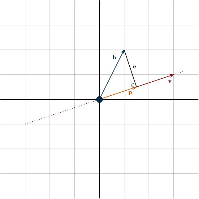
You can see that \(\mathbf{b}\) does not lie in the span of \(\mathbf{v}\) (the dotted line), which represents our column space. But what if we create a vector that is perpendicular to that span and reaches the tip of \(\mathbf{b}\)? This forms a right-angled triangle: the adjacent side is our projected vector \(\mathbf{p}\), which is the closest vector to \(\mathbf{b}\) on that line. You can clearly see that \(\mathbf{p}\) lies in the column space. The perpendicular vector \(\mathbf{e}\) represents the error, how far off we are. When a vector \(\mathbf{b}\) is projected onto a subspace, its projection \(\mathbf{p}\) is the part of \(\mathbf{b}\) that lies along that subspace. The natural question now is: how do we calculate \(\mathbf{p}\)?
In this example, the column space is the span of the vector \(\mathbf{v}\). Notice that \(\mathbf{v}\) is orthogonal to \(\mathbf{e}\), which gives us:
\(\mathbf{v}^{\top} \mathbf{e} = 0\)
Recall from earlier chapters when we discussed covectors and “measuring vectors”, here you can see that idea in action. Taking the dot product with \(\mathbf{v}\) is asking the question: “How much of the input vector lies along the direction of \(\mathbf{v}\)?” The answer is the vector \(\mathbf{p}\).
You can think of the span of \(\mathbf{v}\) as a number line. The tip of the arrow \(\mathbf{p}\) lands on a specific point on that line. That point is exactly what we are looking for, because it tells us how much we need to scale the vector \(\mathbf{v}\) to obtain \(\mathbf{p}\).
If you look closely, you can see that
\(\mathbf{e} = \mathbf{b} \; – \; \mathbf{p}\)
which gives us
\(\mathbf{v}^{\top} (\mathbf{b} \; – \; \mathbf{p}) = 0\)
Since \(\mathbf{p}\) must be a multiple of \(\mathbf{v}\), let that scalar be \(x\). It is the solution we are looking for.
\(\mathbf{v}^{\top} (\mathbf{b} \; – \; x \mathbf{v}) = 0\)
Distributing yields
\(\begin{align*}\mathbf{v}^{\top} \mathbf{b} \; – \; x \mathbf{v}^{\top} \mathbf{v} &= 0 \\\\ x \mathbf{v}^{\top} \mathbf{v} &= \mathbf{v}^{\top} \mathbf{b} \\\\ x &= \frac{\mathbf{v}^{\top} \mathbf{b}}{\mathbf{v}^{\top} \mathbf{v}} \end{align*}\)
Notice that \(\mathbf{v}^{\top} \mathbf{v}\) is a scalar, so dividing by it is perfectly valid (this is where working over a field really matters). Now that we have our scalar, the final step is to construct the vector \(\mathbf{p}\), which is simply \(\mathbf{v}\) scaled by this amount
\(\mathbf{p} = \dfrac{\mathbf{v}^{\top} \mathbf{b}}{\mathbf{v}^{\top} \mathbf{v}} \mathbf{v}\)
Example
Plugging in the actual values from the figure gives
\(\mathbf{p} = \dfrac{1 \cdot 3 + 2 \cdot 1}{3^2 + 1^2} \begin{bmatrix} 3 \\ 1 \end{bmatrix} = \dfrac{5}{10} \begin{bmatrix} 3 \\ 1 \end{bmatrix} = \begin{bmatrix} \frac{3}{2} \\ \frac{1}{2} \end{bmatrix}\)
You might be wondering why we waited so long to introduce this idea. After all, earlier we already talked about sums of subspaces, where any vector could be written uniquely as a part from the first subspace plus a part from the second. So why wasn’t that enough?
The crucial difference is orthogonality. Orthogonality gives us a clean split: moving in one direction has no effect on the other. This independence is exactly what makes projections behave so nicely. Look at the figure again. If you move the error vector \(\mathbf{e}\) up or down, the projection \(\mathbf{p}\) stays exactly the same. That only works because \(\mathbf{e}\) is orthogonal to \(\mathbf{v}\). Now imagine the vectors were not orthogonal, say they form an angle of 80° instead of 90°. If you were to change the length of \(\mathbf{e}\), the other component would no longer stay fixed. The projection \(\mathbf{p}\) would suddenly change as well, growing or shrinking along with \(\mathbf{e}\). Without orthogonality, the components interfere with each other. That coupling makes it much harder to reason about projections and, in particular, to find a closest solution. Orthogonality removes that interference, and that’s why it is essential.
Now, this projection works pretty well for the vector we picked, but couldn’t we build something that does it for any vector? Like, is there a linear transformation that takes the whole space into that subspace?
Projection Transformations via the Outer Product
Our vector space \(V\) comes with a very useful operation: scaling a vector. Let’s make this explicit by defining the map \(s_{\mathbf{v}}\):
\(s_{\mathbf{v}}(c) = c \cdot \mathbf{v}\)
with
\(s_\mathbf{v} : \mathbb{R} \rightarrow V\)
This is simply the linear transformation that scales the fixed vector \(\mathbf{v}\) by a scalar. We also have covectors, which we have encountered earlier. Recall that a covector is nothing more than a linear functional:
\(\varphi: V \rightarrow \mathbb{R}\)
Now we can compose these two linear maps, first evaluating the covector, then scaling the vector:
$$V \xrightarrow{\hspace{0.5cm} \displaystyle \varphi \hspace{0.5cm}} F \xrightarrow{\hspace{0.5cm} \displaystyle s_{\mathbf{v}} \hspace{0.5cm}} V$$
This composition defines a new linear map
\(T: V \longrightarrow V\)
Writing this map explicitly, we obtain
\(T(\mathbf{w}) = s_{\mathbf{v}}(\varphi(\mathbf{w})) = \varphi(\mathbf{w}) \cdot \mathbf{v}\)
Ignoring length (normalization) for the moment, this expression is essentially the projection we derived in the previous section, but now expressed as a linear transformation that acts on any input vector. This transformation takes the entire vector space and maps every vector onto the span of \(\mathbf{v}\), which is a one-dimensional subspace. We therefore call this map a projection transformation.
Using matrix language, this projection transformation corresponds to the projection matrix \(P\), which is formed using the outer product:
\(P = \mathbf{v}\mathbf{v}^{\top}\)
Again, we are temporarily ignoring length. Earlier, in the matrix chapter, the outer product may have seemed like a mysterious kind of vector multiplication that produces a matrix. But now its meaning becomes clear. In the expression \(\mathbf{v}\mathbf{v}^{\top}\), you can think of the covector \(\mathbf{v}^{\top}\) as waiting for an input vector, measuring it, and returning a scalar. That scalar then scales the vector \(\mathbf{v}\). In short:
- measure the input,
- then rescale \(\mathbf{v}\).
This produces a linear transformation, and its corresponding matrix, that maps every vector onto the span of \(\mathbf{v}\), i.e., onto the line defined by \(\mathbf{v}\).
Outer products produce rank-1 matrices. Since the projection maps onto a one-dimensional subspace, the column space of the projection matrix is one-dimensional, which implies that its rank is \(1\).
Now let’s include the length and make the projection fully correct. The projection matrix takes a vector \(\mathbf{b}\) and maps it to its projection \(\mathbf{p}\)
\(\mathbf{p} = P\mathbf{b}\)
Using the projection formula from the previous section, we obtain
\( \begin{align*} \mathbf{p} &= \mathbf{v} \dfrac{ \mathbf{v}^{\top} \mathbf{b}}{\mathbf{v}^{\top} \mathbf{v}} \\\\ &= \Big(\dfrac{1}{\mathbf{v}^{\top} \mathbf{v}} \Big) \mathbf{v} (\mathbf{v}^{\top} \mathbf{b}) \\\\ &= \Big(\dfrac{1}{\mathbf{v}^{\top} \mathbf{v}} \Big) (\mathbf{v} \mathbf{v}^{\top}) \mathbf{b} \\\\ &= \Big(\dfrac{\mathbf{v} \mathbf{v}^{\top}}{\mathbf{v}^{\top} \mathbf{v}} \Big) \mathbf{b} \\\\ &= P\mathbf{b} \end{align*}\)
This shows that the projection matrix is given by
\(P = \dfrac{\mathbf{v} \mathbf{v}^{\top}}{\mathbf{v}^{\top} \mathbf{v}}\)
This is the same result as before, now properly adjusted for length by dividing by \(\mathbf{v}^{\top} \mathbf{v}\).
Example
Looking at the numbers in the figure, we get
\(P = \dfrac{1}{3^2 + 1} \begin{bmatrix} 3 \\ 1 \end{bmatrix} \begin{bmatrix} 3 & 1 \end{bmatrix} = \dfrac{1}{10} \begin{bmatrix} 9 & 3 \\ 3 & 1 \end{bmatrix}\)
Multiplying any vector \(\mathbf{b}\) by this matrix gives the vector on the line that’s closest to \(\mathbf{b}\). To make sure it’s working correctly, let’s try it with the \(\mathbf{b}\) from the figure:
\(\begin{align*} \mathbf{p} &= P\mathbf{b} \\\\ &= \dfrac{1}{10} \begin{bmatrix} 9 & 3 \\ 3 & 1 \end{bmatrix} \begin{bmatrix} 1 \\ 2 \end{bmatrix} \\\\ &= \dfrac{1}{10} \begin{bmatrix} 15 \\ 5 \end{bmatrix} \\\\ &= \begin{bmatrix} \frac{15}{10} \\ \frac{5}{10} \end{bmatrix} \\\\ &= \begin{bmatrix} \frac{3}{2} \\ \frac{1}{2} \end{bmatrix} \end{align*}\)
Projection Onto Higher Dimensional Subspaces
Consider the following figure
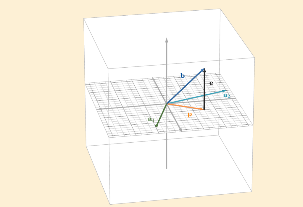
Up to now, we have been projecting onto a line. In this case, however, we are projecting onto a plane (the one with the grid). The natural question is: how do we generalize our projection idea so that it works for any column space? The plane shown in the figure is the column space of the matrix
\(A = \begin{bmatrix} 2 & -6 \\ 5 & -2 \\ 0 & 0 \end{bmatrix}\)
Let the columns of \(A\) be denoted by \(\mathbf{a}_1\) and \(\mathbf{a}_2\). Their span forms the column space. From the figure, we can see that the error vector \(\mathbf{e}\) is orthogonal to both \(\mathbf{a}_1\) and \(\mathbf{a}_2\), and therefore orthogonal to every linear combination of them, that is, to the entire column space. This gives us the conditions
\(\mathbf{a}_1^{\top}\mathbf{e} = \mathbf{0}\)
\(\mathbf{a}_2^{\top}\mathbf{e} = \mathbf{0}\)
Writing these together in matrix form, we get
\(\begin{bmatrix} \text{— } \mathbf{a}_1^{\top} \text{ —} \\ \text{— } \mathbf{a}_2^{\top} \text{ —}\end{bmatrix} \mathbf{e} = \mathbf{0}\)
But the matrix with \(\mathbf{a}_1^{\top}\) and \(\mathbf{a}_2^{\top}\) as rows is simply \(A^{\top}\). So we can write
\(\begin{align*} A^{\top} \mathbf{e} &= \mathbf{0} \\\\ A^{\top}(\mathbf{b} \; – \; \mathbf{p}) &= \mathbf{0} \end{align*}\)
In general, we cannot solve \(A\mathbf{x} = \mathbf{b}\) if \(\mathbf{b}\) is not in the column space of \(A\). The reason is that multiplying by \(A\) always produces a vector in the column space, and if \(\mathbf{b}\) lies outside it, no linear combination of the columns can reproduce it. What we can do instead is solve
\(A\hat{\mathbf{x}} = \mathbf{p}\)
where \(\mathbf{p}\) is the projection of \(\mathbf{b}\) onto the column space, and \(\hat{\mathbf{x}}\) is the combination of columns that produces this closest vector, which gives us
\(\begin{align*} A^{\top}(\mathbf{b} \; – \; A\hat{\mathbf{x}}) &= \mathbf{0} \\\\ A^{\top}\mathbf{b} \; – \; A^{\top}A\hat{\mathbf{x}} &= \mathbf{0} \\\\ A^{\top}A\hat{\mathbf{x}} &= A^{\top}\mathbf{b} \\\\ \hat{\mathbf{x}} &= (A^{\top}A)^{-1} A^{\top}\mathbf{b} \end{align*}\)
Conceptually, this is the same idea as in the one-dimensional line case. The single direction vector \(\mathbf{v}\) has now been replaced by the matrix \(A\), and the scalar term \(\frac{1}{\mathbf{v}^{\top}\mathbf{v}}\) has become the matrix inverse \((A^{\top}A)^{−1}\). This also highlights a key assumption: \((A^{\top}A)^{−1}\) must be invertible. If it is not, we cannot compute the inverse, and the closest solution \(\hat{\mathbf{x}}\) is no longer uniquely defined.
Finally, the projection vector itself is given by
\(\mathbf{p} = A\hat{\mathbf{x}} = A(A^{\top}A)^{-1} A^{\top}\mathbf{b}\)
Since \(\mathbf{p} = P\mathbf{b}\), we see that the projection matrix must be
\(P = A(A^{\top}A)^{-1} A^{\top}\)
Important note. You might be tempted to simplify the projection matrix as follows:
\(A(A^{\top}A)^{-1} A^{\top} \stackrel{?}{=} AA^{-1}(A^{\top})^{-1}A^{\top} = I I = I\)
However, this step is not valid in general. It only works if \(A\) itself is invertible. In our setting, we do not assume that \(A\) is square or invertible. In fact, \(A\) can be rectangular. The only assumption we make is that \(A\) has full column rank, which guarantees that \(A^{\top}A\) is invertible (see below for more info). That special case actually makes sense intuitively. If \(A\) is invertible, then its column space is the entire output space. Projecting onto the column space in that situation means projecting onto everything, so the projection matrix is just the identity.
Now recall that the vector \(\mathbf{b}\) lives in the output space \(\mathbb{R}^m\). This space can be decomposed into two orthogonal subspaces: the column space of \(A\) and the left null space of \(A\), as we saw in the previous chapter. Projection is nothing more than splitting \(\mathbf{b}\) into these two orthogonal components:
\(\mathbf{b} = \mathbf{e} + \mathbf{p}\)
Here, \(\mathbf{p}\) lies in the column space, and \(\mathbf{e}\) lies in the left null space.
If \(\mathbf{b}\) already lies in the column space, then its left–null–space component, the error, is zero. If \(\mathbf{b}\) has components in both subspaces, projection simply discards the error part and keeps the column-space component \(\mathbf{p}\), which is the closest vector we can represent using the columns of \(A\).
Properties of Projection Transformations
If we look more closely at the projection matrix, we can see that it is symmetric
\(P^{\top} = (A(A^{\top}A)^{-1}A^{\top})^{\top} = (A^{\top})^{\top} (A^{\top}(A^{\top})^{\top})^{-1}A^{\top} = A(A^{\top}A)^{-1}A^{\top} = P\)
Another important property is that applying the projection twice is the same as applying it once
\(P^2 = PP = A(A^{\top}A)^{-1}(A^{\top}A)(A^{\top}A)^{-1}A^{\top} = AI(A^{\top}A)^{-1}A^{\top} = A(A^{\top}A)^{-1}A^{\top} = P\)
This also makes perfect sense intuitively. Applying \(P\) projects a vector onto a subspace. Once the vector lies in that subspace, projecting it again has no effect, the vector is already where the projection sends it.
What Does \(A^{\top}A\) Mean?
The matrix \(A^{\top}A\) and its sibling \(AA^{\top}\) appear everywhere in linear algebra. From Least Squares (which we will discuss shortly), to the Singular Value Decomposition, to PCA, all fundamental and highly relevant machine learning tools.
Why is pairing a linear transformation with its adjoint so powerful? What is it actually doing?
To answer this, we need to start at the beginning: our basis. The choice of basis is up to us, so we are perfectly free to choose a skewed basis, like the one below.
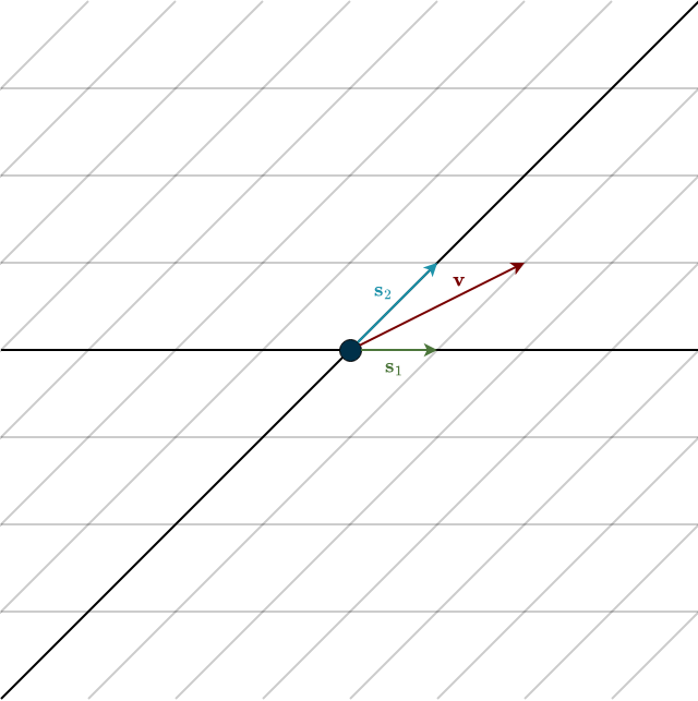
Let the skewed basis vectors be
\(\mathbf{s}_1 = \begin{bmatrix} 1 \\ 0 \end{bmatrix}, \hspace{0.5cm} \mathbf{s}_2 = \begin{bmatrix} 1 \\ 1 \end{bmatrix}\)
written in standard coordinates. In their own coordinate system, they would look like the standard basis looks to us: \((1,0)\) and \((0,1)\). But geometrically, they are clearly not orthogonal. In standard coordinates, they sit at a 45° angle. And just to confirm
\(\mathbf{s}_1^{\top}\mathbf{s}_2 = \begin{bmatrix} 1 & 0 \end{bmatrix}\begin{bmatrix} 1 \\ 1 \end{bmatrix} = 1\)
So the numbers confirm what we see: they are not orthogonal.
Remember, a basis exists to span the space. That means we can build any vector \(\mathbf{v}\) as
\(\mathbf{v} = v_1 \cdot \mathbf{s}_1 + v_2 \cdot \mathbf{s}_2 = v_1 \cdot \begin{bmatrix} 1 \\ 0 \end{bmatrix} + v_2 \cdot \begin{bmatrix} 1 \\ 1 \end{bmatrix} = \begin{bmatrix} v_1 + v_2 \\ v_2 \end{bmatrix}\)
Notice something important: The first coordinate mixes both basis coefficients. That’s an issue. Our goal in projection problems is to split error from projection. But here, changing one coordinate affects the other. We cannot isolate directions cleanly because we have no orthogonality.
In the animation, the red vector is expressed in this skewed basis. When we move it purely “up” in the standard grid, both skewed components change. There’s no clean separation. The directions interfere with each other.
At this point, you might object: But in their own coordinates the vectors are \((1,0)\) and \((0,1)\). Their dot product is zero there, so aren’t they orthogonal? And if the red vector moves diagonally, don’t we isolate the coordinates just fine?
See! Only one coordinate changes. So we can split error from projection. Right?
There are two key issues here. First, while you can split coordinates algebraically (i.e., using mathematical notation), that does not make the geometric vectors perpendicular. Geometry is not fixed by how we write numbers. Orthogonality is a geometric concept, not a coordinate trick. We need orthogonality to guarantee the closest possible projection vector \(\mathbf{p}\) to \(\mathbf{b}\). Without orthogonality, we do not get minimal distance behavior.
Second, and more fundamentally, orthogonality is not about coordinates. It is about the inner product. Coordinates do not define angles. Inner products do. Angles and lengths are determined by the inner product, not by how vectors look as lists of numbers. Changing basis does not change geometry. It only changes representation. The vectors themselves did not magically rotate to 90° just because we changed coordinates. So why do they appear orthogonal in their own coordinate system?
Because we incorrectly kept using the standard dot product:
\(\langle \mathbf{x}, \mathbf{y} \rangle = \mathbf{x}^{\top}\mathbf{y}\)
That formula only works in an orthonormal basis. When we changed to a skewed basis, we silently pretended it was still orthonormal. That’s why the computation falsely suggests orthogonality. The inner product itself exists independently of coordinates. What changes under a new basis is how we compute it.
Write two vectors in the skewed basis:
\(\mathbf{u} = u_1 \mathbf{s}_1 + u_2 \mathbf{s}_2, \hspace{0.5cm} \mathbf{v} = v_1 \mathbf{s}_1 + v_2 \mathbf{s}_2\)
Their inner product becomes
\(\begin{align*} \langle \mathbf{u}, \mathbf{v} \rangle &= u_1v_1 (\mathbf{s}_1 \cdot \mathbf{s}_1) + u_1v_2 (\mathbf{s}_1 \cdot \mathbf{s}_2) + u_2v_1 (\mathbf{s}_2 \cdot \mathbf{s}_1) + u_2v_2 (\mathbf{s}_2 \cdot \mathbf{s}_2)\end{align*}\)
If the basis were orthonormal, the cross terms would vanish and the diagonal terms would be \(1\). That would reduce to
\(\langle \mathbf{u}, \mathbf{v} \rangle = u_1v_1 + u_2v_2\)
This is the standard dot product we are used to. But our basis is not orthonormal. Computing the dot products in standard coordinates gives:
\(\mathbf{s}_1 \cdot \mathbf{s}_1 = 1, \hspace{0.5cm} \mathbf{s}_1 \cdot \mathbf{s}_2 = 1, \hspace{0.5cm} \mathbf{s}_2 \cdot \mathbf{s}_2 = 2\)
So the inner product becomes
\(\langle \mathbf{u}, \mathbf{v} \rangle = u_1v_1 + u_1v_2 + u_2v_1 + 2 \cdot (u_2v_2)\)
This looks clearly different, but we can write it cleanly as
\(\mathbf{u}^{\top} G \mathbf{v} = \begin{bmatrix} u_1 & u_2\end{bmatrix} \begin{bmatrix} \mathbf{s}_1 \cdot \mathbf{s}_1 & \mathbf{s}_1 \cdot \mathbf{s}_2 \\ \mathbf{s}_2 \cdot \mathbf{s}_1 & \mathbf{s}_2 \cdot \mathbf{s}_2 \end{bmatrix} \begin{bmatrix} v_1 \\ v_2 \end{bmatrix}\)
where
\(G = \begin{bmatrix} 1 & 1 \\ 1 & 2 \end{bmatrix}\)
This matrix \(G\) is the Gram matrix. If the basis were orthonormal, then \(G=I\). But in a skewed basis, \(G\) compensates for non-orthogonality. Now, computing in the skew coordinates:
\(\mathbf{s}_1^{\top} \begin{bmatrix} 1 & 1 \\ 1 & 2 \end{bmatrix} \mathbf{s}_2 = \begin{bmatrix} 1 & 0 \end{bmatrix} \begin{bmatrix} 1 & 1 \\ 1 & 2 \end{bmatrix} \begin{bmatrix} 0 \\ 1 \end{bmatrix} = \begin{bmatrix} 1 & 0 \end{bmatrix} \begin{bmatrix} 1 \\ 2 \end{bmatrix} = 1\)
Now everything matches. They are not orthogonal, even in their own coordinates, once we measure correctly. So the matrix \(G\) didn’t change vectors. It changes how we measured them. Does that sound familiar?
Recall the adjoint: it lets us either
- transform a vector and then measure it, or
- leave the vector alone but adjust how we measure it.
The Gram matrix is doing exactly that. It answers: What matrix do I insert so that computing in skew coordinates gives the same answer as computing in standard coordinates? Now we’re ready for the bigger picture.
A general linear transformation \(T\) changes geometry. It stretches some directions, squashes others, and destroys orthogonality. After applying \(T\), the standard dot product no longer reflects the original geometry correctly. So we have two choices:
- Physically undo the distortion. (Which often isn’t realistic.)
- Adjust how we measure.
\(A^{\top}A\) does the second.
In matrix form,
\(A^{\top}A = \begin{bmatrix} \text{— } \mathbf{a}_1^{\top} \text{ —} \\ \text{— } \mathbf{a}_2^{\top} \text{ —}\end{bmatrix} \begin{bmatrix} | & | \\ \mathbf{a}_1 & \mathbf{a}_2 \\ | & | \end{bmatrix} = \begin{bmatrix} \mathbf{a}^{\top}_1\mathbf{a}_1 & \mathbf{a}^{\top}_1 \mathbf{a}_2 \\ \mathbf{a}^{\top}_2\mathbf{a}_1 & \mathbf{a}^{\top}_2\mathbf{a}_2\end{bmatrix} = G\)
It is the Gram matrix of the columns of \(A\). It records how lengths and angles changed under the transformation. Its inverse, \((A^{\top}A)^{−1}\), rebalances the measurements. If a direction was stretched, it down-weights it. If a direction was squashed, it up-weights it. In short: \(A^{\top}A\) tells us how space was warped. \((A^{\top}A)^{−1}\) compensates for that warp.
A simple analogy might help: Imagine a metal rod measuring 15 cm. A transformation stretches it by 2. Now it measures 30 cm. You could physically stretch the rod and measure again. Or, knowing the stretch factor, you could simply double the ruler. That’s what \(A^{\top}A\) does. It adjusts the ruler instead of the object.
Now, what does \(AA^{\top}\) do then?
This one is simpler. Recall projection onto a single vector \(\mathbf{a}\):
\(\mathbf{a}\mathbf{a}^{\top}\)
It measures a vector, produces a scalar, and rebuilds the projection along \(\mathbf{a}\) (ignoring normalization). Now extend this idea to multiple directions:
\(AA^{\top} = \sum^{n}_{k = 1} \mathbf{a}_k \mathbf{a}_k^{\top}\)
Each term acts like a projection operator along one column of \(A\). The sum rebuilds the full projection. If the columns of \(A\) are orthonormal, then
\(P = AA^{\top}\)
because \(A^{\top}A=I\). \(T\) didn’t change the geometry, so we don’t need to make any adjustments. But if the columns are not orthonormal, the components interfere, just like in our skewed basis example. That’s why the full projection formula becomes
\(P = A(A^{\top}A)^{-1}A^{\top}\)
Example
Consider the following figure
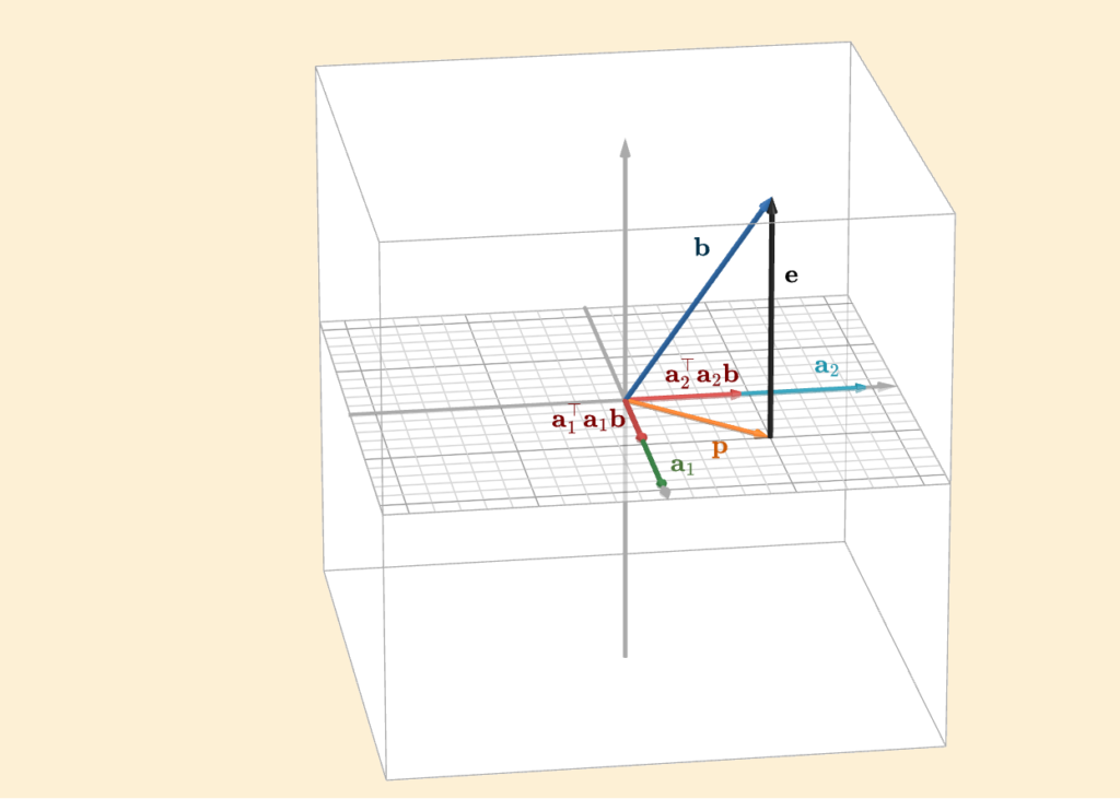
The column space, together with the columns \(\mathbf{a}_1\) and \(\mathbf{a}_2\), comes from the matrix
\(A = \begin{bmatrix} 1 & 0 \\ 0 & 1 \\ 0 & 0\end{bmatrix}\)
Very creative, I know.
Its column space is simply the plane shown in the figure (the one with the grid). Now suppose we have a vector \(\mathbf{b}\) that does not lie in this column space, and we would like to project it onto it. In this setting, we can clearly see what \(AA^{\top}\) does:
\(AA^{\top} = \mathbf{a}_1^{\top}\mathbf{a}_1 + \mathbf{a}_2^{\top}\mathbf{a}_2 = \begin{bmatrix} 1 \\ 0 \\ 0 \end{bmatrix} \begin{bmatrix} 1 & 0 & 0\end{bmatrix} + \begin{bmatrix} 0 \\ 1 \\ 0 \end{bmatrix} \begin{bmatrix} 0 & 1 & 0\end{bmatrix} = \begin{bmatrix} 1 & 0 & 0\\ 0 & 0 & 0 \\ 0 & 0 & 0\end{bmatrix} + \begin{bmatrix} 0 & 0 & 0\\ 0 & 1 & 0 \\ 0 & 0 & 0\end{bmatrix} = \begin{bmatrix} 1 & 0 & 0\\ 0 & 1 & 0 \\ 0 & 0 & 0\end{bmatrix}\)
\(\mathbf{p} = P\mathbf{b} = \begin{bmatrix} 1 & 0 & 0\\ 0 & 1 & 0 \\ 0 & 0 & 0\end{bmatrix} \begin{bmatrix} \frac{1}{2} \\ \frac{1}{2} \\ 1 \end{bmatrix} = \begin{bmatrix} \frac{1}{2} \\ \frac{1}{2} \\ 0 \end{bmatrix}\)
Each term in this sum contributes one component of the projection vector \(\mathbf{p}\), as illustrated in the figure. One term projects onto the direction of \(\mathbf{a}_1\), the other onto \(\mathbf{a}_2\). Adding them together gives the full projection \(\mathbf{p}\).
And this is the key idea: just as we decompose \(\mathbf{b}\) into projection plus error, we can decompose the projection itself into parts, one along each basis direction of the column space. However, there is an important caveat. This clean decomposition works only because the columns of \(A\) are already orthonormal. If the columns are not orthonormal, we run into the same issue as before: adjusting one component influences the others. The directions are no longer independent, so we cannot split the projection cleanly into separate, non-interfering parts. Even if the columns are orthogonal, they can still stretch or shrink the space if they don’t have unit length.
In general, a transformation \(T\) distorts Euclidean geometry. It stretches, compresses, or skews space, and as a result, the columns of \(A\) are no longer orthonormal. That is precisely why the projection formula includes \((A^{\top}A)^{−1}\). This term compensates for the geometric distortion, restoring the correct scaling and independence of directions so that the projection is once again geometrically meaningful.
Properties of \(A^{\top}A\)
\(A^{\top}A\) has several very useful properties, which I’ll briefly mention here. First of all, it is invertible whenever \(A\) has full column rank. (Otherwise, this whole page of explanation would have been a bit of a waste of time.) I won’t go into all the details here, but if you think about the null space and how it relates to injectivity of a linear transformation, you can work it out yourself. Or, if you are lazy, you can always just look it up.
The matrix \(A^{\top}A\) is square, since it comes from composing \(T\) with its adjoint \(T^*\). If \(T: V \rightarrow W\) and \(T^*:W \rightarrow V\), then the composition \(T^*T:V \rightarrow V\). In other words, it maps a vector space back to itself, which means its matrix representation must be square. Recall that a linear transformation that maps a space to itself is called an operator.
Another nice property is that \(A^{\top}A\) is symmetric (With \(K = T^*T\) then \(K = K^*\)). This is easy to see:
\((A^{\top}A)^{\top} = A^{\top}(A^{\top})^{\top} = A^{\top}A\)
(It is also positive definite, but we’ll leave that discussion for a later chapter.)
Least Squares
At last! After everything we’ve learned so far, after all the struggle and challenges, we’ve finally arrived at our first real piece of statistical learning, or machine learning, algorithm. Let’s start with the very basics. Consider the following figure, showing some simple lines, much like the ones you might have seen in school
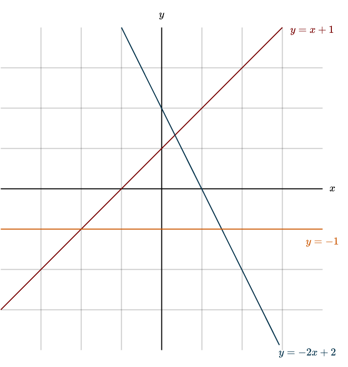
Its definition is
\(y = b + mx\)
Here, \(m\) represents the slope of the line, and \(b\) is the y-intercept, which is the point where the line crosses the y-axis. Changing these parameters changes the line itself: think of \(m\) as rotating the line, and \(b\) as shifting it up or down. Now that we’re comfortable with line terminology, let’s move on to a real-world example.
Imagine you work at a real estate agency and you are given a small dataset:
| House | Size(\(x\)) (\(\times 100\text{m}^2\)) | Price(\(y\)) (\(\times 100.000€\)) |
| 1 | 0.5 | 0.1 |
| 2 | 1.0 | 1.2 |
| 3 | 1.5 | 2.1 |
| 4 | 2.0 | 1.8 |
| 5 | 2.5 | 2.2 |
| 6 | 3.0 | 3.9 |
It relates the size of a house to its price. Your task is to build a model, a kind of “machine”, that can predict the price of a house based on its size. How do we start? The first step is simple: plot all of the points on a graph.
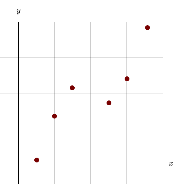
You can see that there’s clearly some kind of relationship between the size of a house and its price. In general, the bigger the house, the more expensive it tends to be. But this dataset isn’t perfect. There’s noise in the data. That means there are factors we’re not accounting for, things like location, age, condition, or type of house, that also influence the true price. On top of that, how accurately the data was collected (or how poorly) also adds to the noise. Small measurement discrepancies are completely normal. That’s why the data points don’t lie perfectly on a straight line. That’s why we have error. Because of this, we can’t expect to find a perfectly fitting solution. There will always be some error. Our job, given the dataset, is to make that error as small as possible. How do we do that?
Simple, we draw a line that generally follows the overall trend.
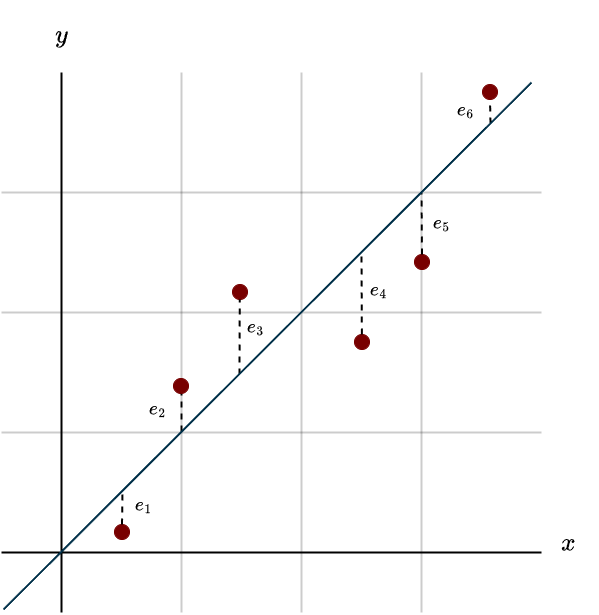
Now you can see the error (often called the residual) for each data point. It’s the vertical dotted line from the point down (or up) to our fitted line, our model. Our task is to tweak the slope and the y-intercept so the overall error becomes as small as possible. When we adjust the line, it might fit better in some places and worse in others, so the goal is to find the sweet spot where the total error across all the data points is minimized. We could try guessing and adjusting by trial and error, but that would take forever. Instead, we use mathematics to compute the best possible fit directly.
Recall the equation of a line:
\(y = b + mx\)
To avoid confusion with the notation of solving linear systems, we’ll rename the parameters. Instead of \(m\) and \(b\), we’ll use:
- \(w_1\) for the y-intercept
- \(w_2\) for the slope
So the equation becomes:
\(y = w_1 + w_2 x\)
In an ideal world, our line would pass exactly through every point. That would give us one equation per data point:
\(\begin{align} 0.1 &= w_1 +w_2 \cdot 0.5 \\ 1.2 &= w_1 + w_2 \cdot 1.0 \\ 2.1 &= w_1 + w_2 \cdot 1.5 \\ 1.8 &= w_1 + w_2 \cdot 2.0 \\ 2.2 &= w_1 + w_2 \cdot 2.5 \\ 3.9 &= w_1 + w_2 \cdot 3.0 \end{align}\)
This practically screams systems of linear equations, so let’s translate it into our familiar matrix notation.
\(A \mathbf{x} = \mathbf{b} \hspace{0.5cm} \Longleftrightarrow \hspace{0.5cm} \begin{bmatrix} 1 & 0.5 \\ 1 & 1.0 \\ 1 & 1.5 \\ 1 & 2.0 \\ 1 & 2.5 \\ 1 & 3.0\end{bmatrix} \begin{bmatrix} w_1 \\ w_2 \end{bmatrix} = \begin{bmatrix} 0.1 \\ 1.2 \\ 2.1 \\ 1.8 \\ 2.2 \\ 3.9 \end{bmatrix}\)
Notice that one column of the matrix consists entirely of \(1\)s. This comes from the fact that \(w_1\) always remains alone, that is, it is only scaled by \(1\). In addition, the first entry of the solution vector corresponds to the y-intercept, and the second to the slope.
Also note that the matrix is clearly not square, so we can throw invertibility, and with it the possibility of an exact or perfect solution, out the window, though we already knew that. We also have more rows than columns (\(m>n\)). If you remember the chapter on solving linear systems, this means the system has a unique solution only if \(\mathbf{b}\) lies in the column space of \(A\). However, this column space is so thin that finding a love letter in your mailbox instead of bills is more likely than \(\mathbf{b}\) landing in it. But this is exactly the kind of problem we’ve learned to handle in this chapter. The columns of \(A\) are independent, giving us full column rank. That, in turn, allows us to use projection to find the closest solution.
Two seemingly different problems, fitting a line through many points and projecting a vector onto a subspace, share the same underlying solution. Same stone, just viewed from a different angle. Take a moment to appreciate how naturally this solution emerged. You could also derive it using calculus, but that’s far less fun.
To actually calculate the solution, we compute
\((A^{\top}A)^{-1}A^{\top}\mathbf{b}\)
You could work this out by hand, but the numbers get fairly ugly, so it’s much easier to let a computer handle it. (Note that we’re solving for \(\mathbf{x}\) here, not for the projection matrix.) From the example above, we obtain
\(\mathbf{x} = \begin{bmatrix} -\frac{43}{150} \\ \frac{31}{25} \end{bmatrix} \approx \begin{bmatrix} -0.29 \\ 1.24 \end{bmatrix}\)
This gives the following equation for the line
\(y = 1.24x \; – \; 0.29\)
Once we’ve built our model, in this case, our fitted line, we can actually start using it. Imagine picking a random house, measuring its size, and plugging that number into our model (the equation above). The model would then predict a price based on the data it learned from. You can even visualize this process. Plot the line, then go to the size of your chosen house on the x-axis. From there, move straight up until you hit the line. Then move straight across to the y-axis. The point where you land is the predicted price. That’s your model in action.
In many real-world scenarios, the relationship between input and output isn’t strictly linear, it can be far more complex. Take the relationship between study time and test scores, for example. At first, as you spend more time studying, your performance tends to improve rapidly. However, after many hours, the gains become smaller and more incremental. So how can we model this kind of complexity? How can we effectively capture nonlinearity? Simple: instead of fitting a straight line, we fit a curve, specifically, a parabola. We modify our model to:
\(y = w_1 + w_2x + w_3x^2\)
The setup is almost the same as before, except we’ve added the \(x^2\) term. Now you might be thinking: Wait, this is linear algebra. And \(x^2\) definitely isn’t linear.
That’s a good observation, but here’s the key point: the model is still linear in the parameters. The unknowns \(w_1, w_2\) and \(w_3\) all appear linearly. We’re not squaring the weights, we’re squaring the input. That means fitting the best parabola is still a linear algebra problem. The difference is that we’re now fitting a curve instead of a rigid straight line. But conceptually, nothing changes. We are still searching for the parameter values that minimize the total error. The roles of the parameters are just a bit different now:
- \(w_1\) is still the y-intercept.
- \(w_2\) controls the linear tilt of the curve.
- \(w_3\) introduces curvature, it bends the line upward or downward, depending on its sign.
Solving this works almost exactly the same way as before. The only structural change is in our matrix \(A\): instead of two columns (for \(x\) and the constant \(1\)), we now have three columns, one additional column corresponding to the \(x^2\) term. Plotting a parabola in this context usually looks something like this
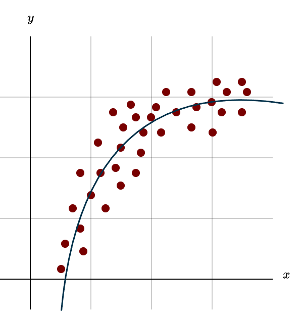
This figure shows the example of study time versus test results. If we tried to fit a simple straight line to this data, it would likely perform poorly because the relationship clearly isn’t purely linear. But why stop at a parabola? Why not add \(x^3\), \(x^4\), or even \(x^5\)? The higher the powers we include, the more flexible, or “bendier”, the model becomes.
In general, a \(k\)-degree polynomial can change direction (go from decreasing to increasing, or vice versa) up to \(k−1\) times. A straight line can’t change direction at all. A parabola can change direction once. A cubic polynomial can do it twice, and so on. At this point, you might be thinking: Perfect. Let’s just go up to \(x^{100}\) so we can capture the data perfectly. Then our model has to perform perfectly, right?
Not quite. In statistics and machine learning, there’s a fundamental trade-off between bias and variance, and this connects directly to a concept called overfitting. I won’t go into full detail here, we’ll cover it properly in the machine learning course, but the short version is this: overfitting is bad. Overfitting is like memorizing last year’s exam answers word for word. You might do great if the exact same questions show up again. But the moment the questions change, you’re stuck, because you never actually understood the underlying concepts. You just memorized the answers.
What Are We Actually Minimizing?
Clearly, we want to make the total error \(E\) as small as possible, where the total error is just the sum of all the small errors coming from each data point. Each of those small errors is one entry of the error vector \(\mathbf{e}\). Calculus tells us that we need to square the error terms.
\(E = \sum_{k=1}^m e_k^2 = e_1^2 + e_2^2 + \dots + e_m^2\)
Why? Because squaring them makes the function differentiable throughout, which lets us compute the derivative much more easily, unlike when we use absolute values. So, we square the errors. And we want less of that, preferably the least possible sum of squared errors. Get it? Least squares? That’s actually where the name comes from. Anyway…
From the linear algebra point of view, the squaring comes from a slightly different angle. Our job is to minimize
\(E = ||A\mathbf{x} \; – \; \mathbf{b}||^2\)
Now you might say: Why are we minimizing \(A\mathbf{x}−\mathbf{b}\)? The error is clearly \(\mathbf{e}= \mathbf{b} \;− \; \mathbf{p}\), so why are we even looking at this? And why do we square it? If we want to minimize the length of the error vector, couldn’t we just use the regular norm instead of the squared one?
I get where you’re coming from. Let me explain. Consider the following figure
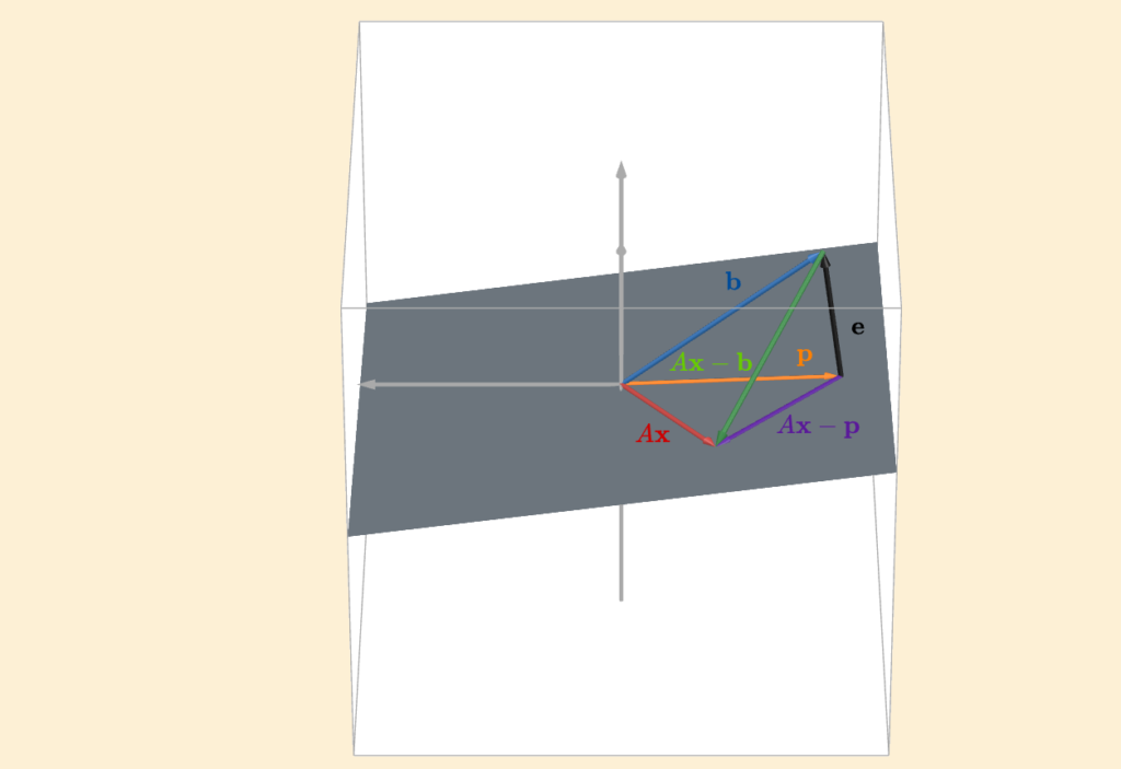
There’s a lot going on here, so let’s unpack it step by step. First, focus on \(A\mathbf{x}\). We know that multiplying by \(A\) transforms any vector and places it inside the column space of \(A\). That’s the only thing \(A\) can do. It takes whatever vector you give it and produces something that lives in its column space. In this context, \(A\mathbf{x}\) represents some projection vector. Think of it like positioning a line however we want in the “fit a line” problem. We can choose different \(\mathbf{x}\), and each choice gives us a different \(A\mathbf{x}\). But most of those choices won’t be optimal. Now look at \(A\mathbf{x} \; – \; \mathbf{b}\). That’s the error vector corresponding to whatever random projection we picked. (Since we can write \(\mathbf{b} = A\mathbf{x} + \mathbf{e}_{\text{new}}\) it follows that \(\mathbf{e}_{\text{new}} = \mathbf{b} \; – \; A\mathbf{x}\) and since the norm does not care about direction we can simply focus on \(||A\mathbf{x} \; – \; \mathbf{b}||\))
Notice something important: this new error vector is longer than the orthogonal error vector (the one from the best projection). In other words, it contains more error. Next, look at \(A\mathbf{x} \; – \; \mathbf{p}\). This is the difference between our randomly chosen projection \(A\mathbf{x}\) and the perfect projection \(\mathbf{p}\). If you look at the figure, do you see the right angled triangle? The one formed by the green, black, and purple vectors?
That triangle is the key. By Pythagoras, we get
\(||A\mathbf{x} \; – \; \mathbf{b}||^2 = ||A\mathbf{x} \; – \; \mathbf{p}||^2 + ||\mathbf{e}||^2\)
And this is exactly where the squaring comes from in the linear algebra perspective. Now notice that there are two kinds of errors in this equation.
First, there’s \(\mathbf{e}\). This error is fixed. No matter what we do, it won’t disappear. It comes from how the dataset was created, missing factors, measurement noise, randomness, and so on. That’s just reality.
Second, there’s \(A\mathbf{x} \; – \; \mathbf{p}\). This is the error we can control. It exists because we chose the wrong projection, or, in the line-fitting picture, because we placed the line badly. A wrong projection means a longer error vector, which means worse performance. So why do we minimize \(||A\mathbf{x} \; – \; \mathbf{b}||^2\)? Because minimizing this quantity forces
\(A\mathbf{x} \; – \; \mathbf{p} = \mathbf{0}\)
When that happens, we’re left with
\(\mathbf{e} = \mathbf{b} \; – \; \mathbf{p}\)
which is the minimal possible error. It’s not that \(\mathbf{e} = \mathbf{b} \; – \; \mathbf{p}\) isn’t important, it absolutely is. It’s just that this already represents the best-case scenario. And we arrive at that best case precisely by minimizing \(||A\mathbf{x} \; – \; \mathbf{b}||^2\). The animation below shows this minimization in action.
Summary
- If \(A\mathbf{x}=\mathbf{b}\) has no exact solution, we project \(\mathbf{b}\) onto the column space of \(A\). This gives the closest possible vector \(\mathbf{p}\) in that space.
- Finding this closest solution requires orthogonality. We split \(\mathbf{b}\) into two clean parts: \(\mathbf{b} = \mathbf{p} + \mathbf{e}\), where \(\mathbf{p}\) is in the column space and the error \(\mathbf{e}\) is in the left null space.
- In matrix language, multiplying a column vector \(\mathbf{u}\) by a row vector \(\mathbf{v}^{\top}\) produces a rank-1 matrix through the outer product \(\mathbf{u}\mathbf{v}^{\top}\). It measures along \(\mathbf{v}\) and scales in direction \(\mathbf{u}\).
- If \(\mathbf{u} = \mathbf{v} \) and both are unit vectors, then \(\mathbf{u}\mathbf{u}^{\top}\) is the projection matrix onto the span of that vector. If they are not unit vectors, we can normalize them by dividing by their length.
- A projection matrix \(P\) represents a transformation that maps the entire space onto the column space. Every vector gets “pulled down” to its closest point in that subspace.
- Projecting onto a higher-dimensional subspace is similar to projecting onto a line, except now we must account for multiple independent directions instead of just one.
- If the transformation preserves geometry (meaning it keeps orthogonality intact), then \(A^{\top}A=I\), and the projection matrix simplifies to \(P=AA^{\top}\). In this case, we can think of building the projection step by step: each \(\mathbf{a}\mathbf{a}^{\top}\) contributes one directional component along the column space of \(A\), and their sum gives the full projection matrix.
- If the transformation does not preserve orthogonality, then \((A^{\top}A)^{-1}\) adjusts how we measure lengths and angles. It compensates for the distortion so we can still reason correctly about orthogonality. In the general case, the projection matrix is \(P = A(A^{\top}A)^{-1}A^{\top}\)
- The projection matrix \(P\) is symmetric, and applying it multiple times gives the same result: once a vector is in the column space, projecting again does nothing.
- The matrix \(A^{\top}A\) is symmetric and invertible as long as \(A\) has full column rank.
- Least squares fits a line or curve by minimizing squared error.
- Geometrically, fitting a line (or curve) and projecting a vector onto a subspace are the same problem. In both cases, we minimize \(||A\mathbf{x} \; − \; \mathbf{b}||^2\)