Transpose, Dual Spaces, Adjoints, and Symmetric Matrices
What does transposing a matrix actually mean?
Transposing a matrix is central to linear algebra and machine learning. On the surface, it simply means exchanging the rows and columns of a matrix, but at a deeper mathematical level there is much more going on. Every vector space has a corresponding dual space. Vectors live in the vector space, while covectors live in the dual space. Linear transformations act on vectors, and every linear transformation has a corresponding transpose transformation that acts on covectors. With the help of the inner product, we can move between vectors and covectors. This connection allows us to define the adjoint transformation, which in turn leads naturally to the concept of self-adjoint operators. In matrix form, self-adjoint transformations are represented by symmetric matrices.
Don’t worry if this sounds more complicated than the previous topics. There is a lot to unpack here, and we will take it slowly, building up the ideas step by step.
Linear Functional
Imagine we want to ask questions about vectors, measure them in different ways. For example: What is the x-component of this vector? What is the y-component? How well is it aligned with another vector? How much of it lies in a given direction? What does its projection onto some fixed direction look like? For this, we need a tool that measures vectors, a function that takes in a vector and spits out a number. This is where linear functionals come in. They are a special kind of linear transformation in which the output space is the field \(\mathbb{R}\); instead of returning a vector, they return a number.
A linear functional on \(V\) is a linear map from \(V\) to \(F\). In other words, a linear functional is an element of \(\mathcal{L}(V, F)\)
Example
Imagine we want to extract the second coordinate of a vector in \(V=\mathbb{R}^2\). Then the corresponding linear functional \(\varphi\) looks like this:
\(\varphi(\mathbf{v}) = \varphi((v_1, v_2)) = 0 \cdot v_1 + 1 \cdot v_2 = v_2\)
It takes in a vector and spits out a number. It measures the vector, specifically, it picks out the second coordinate. Nothing more, nothing less.
Now there isn’t just one question we can ask about vectors, but infinitely many. If we take all of these “measurement devices” that can ask questions about vectors in \(V\) and collect them into a set, we obtain a vector space. This vector space is special, so it gets a cool name.
Dual Space
The dual space of \(V\), denoted by \(V’\), is the vector space of all linear functionals on \(V\). In other words:
\(V’ = \mathcal{L}(V, F)\).
We call the elements of this dual space dual vectors, or covectors. These are the linear functionals. Be careful: covectors and vectors are two different kinds of objects. A vector is a mathematical object that can represent many things, such as a list of numbers or a geometric arrow, while a covector is a function that “eats” a vector. It measures it. They are not the same.
We have the following interesting fact about the dual space.
Suppose \(V\) is finite-dimensional. Then \(V’\) is also finite-dimensional and
\(\text{dim}(V) = \text{dim}(V’)\)
Remember that the dimension of a vector space is defined via its basis, specifically, it is the number of basis vectors. So there must be some connection between the basis of \(V\) and the basis of \(V′\).
Dual Basis
It would be nice if we could construct a corresponding dual basis for \(V’\) from the basis of our vector space \(V\). Then, if we were to change the basis of \(V\), the dual basis would change along with it. It should also be simple and efficient, making it easier to work with later on. The definition below satisfies all of these requirements:
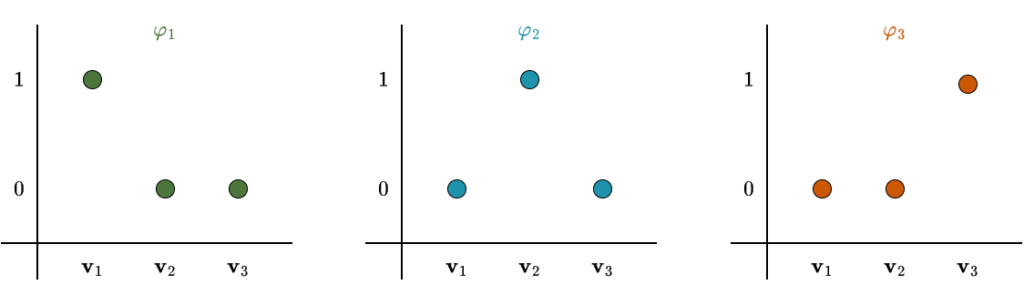
If \(\mathbf{v}_1, \dots, \mathbf{v}_n\) is a basis of \(V\), then the dual basis of \(\mathbf{v}_1, \dots, \mathbf{v}_n\) is the list \(\mathbf{\varphi}_1, \dots, \mathbf{\varphi}_n\) of elements of \(V’\), where each \(\varphi_j\) is the linear functional on \(V\) such that
\(\varphi_j(v_k) = \begin{cases} 1 & \text{if } k = j, \\ 0 & \text{if } k \neq j. \end{cases}\)
This definition may look strange at first, but don’t worry, it is actually quite easy to understand once you see what it is doing. Recall that linear functionals are functions: they take vectors as input and return numbers. After choosing a basis for a vector space \(V\), every basis vector \(\mathbf{v} \in V\) has a corresponding dual basis vector \(\varphi \in V’\). This linear functional evaluates to \(1\) on its associated basis vector and to \(0\) on all the others. For vectors that are not basis vectors, its output will generally be some number determined by linearity. If \(V\) had three basis vectors, the figure below would illustrate this behavior.
At this point, you might be asking: Why do we need this? Why must the value be \(1\) when the indices match? Why must it be \(0\) otherwise? To answer these questions, we need to step back and recall the motivation behind this course. At the beginning, I mentioned that we translate real-world objects, geometric vectors, housing-price data, and so on, into \(\mathbb{R}^n\) using a chosen basis. This translation allows us to apply general algorithms and, most importantly, let the computer handle the calculations. Linear algebra is powerful precisely because it gives us a generic framework that works across many different problem domains.
The first step in this process is converting vectors from the original problem into vectors in \(\mathbb{R}^n\). But vectors in \(\mathbb{R}^n\) are just lists of numbers, coordinates. So we need a tool that takes a vector and produces numbers. More precisely, we need a function that “measures” a vector and returns a scalar. That is exactly what a linear functional does.
Now let’s focus on how this works in practice. Once we choose a basis, every vector can be written as a linear combination of basis vectors:
\(\mathbf{v} = a_1 \cdot \mathbf{v}_1 + \dots + a_n \cdot \mathbf{v}_n\)
where \(\mathbf{v}_1, \dots, \mathbf{v}_n\) are the basis vectors and \(a_1, \dots, a_n\) are the coordinates, the numbers that appear in the coordinate representation. But how do we extract these coordinates? This is where the dual basis comes in. Suppose we want to extract the first coordinate \(a_1\). To do this we apply the first dual basis vector \(\varphi_1\):
\(\varphi_1(\mathbf{v}) = \varphi_1(a_1 \cdot \mathbf{v}_1 + \dots + a_n \cdot \mathbf{v}_n)\)
Because \(\varphi_1\) is a linear functional, we can use additivity and homogeneity:
\(\varphi_1(\mathbf{v}) = a_1 \cdot \varphi_1(\mathbf{v}_1) + \dots + a_n \cdot \varphi_1(\mathbf{v}_n)\)
Now pay close attention, this is the key point. By definition, the dual basis vector \(\varphi_1\) evaluates to \(1\) on \(\mathbf{v}_1\) and to \(0\) on all other basis vectors. Therefore,
\(\varphi_1(\mathbf{v}) = a_1 \cdot \underbrace{\varphi_1(\mathbf{v}_1)}_{ =\;1} + \dots + a_n \cdot \underbrace{\varphi_1(\mathbf{v}_n)}_{=\;0} = a_1\)
This is exactly what we wanted: \(\varphi_1\) extracts the first coordinate. If we changed the definition and made \(\varphi_1(\mathbf{v}_1) = 2\), then the result would be \(2 \cdot a_1\), a scaled coordinate rather than the original one. If \(\varphi_1\) evaluated to something nonzero on the other basis vectors, those extra terms would not disappear, and we would end up with a messy mixture of coordinates.
This is why the dual basis is defined the way it is. Of course it is not the only possible choice, any set of linearly independent linear functionals that spans the dual space would work. But this particular choice makes computations clean, direct, and intuitive.
An analogy may help. Imagine you ate an excellent pizza and want to recreate it. The pizza is a combination of ingredients: salt, water, flour, yeast, and so on. Think of these ingredients as the basis vectors. The pizza itself is a linear combination of them. The coordinate representation tells you how much of each ingredient was used: \(a_1\) units of salt, \(a_2\) units of water, and so forth.
To recreate the recipe, you need a way to measure each ingredient separately. That requires a different measuring cup for each ingredient: one that measures only salt, one that measures only flour, and so on. These measuring cups are the dual basis vectors. Each one ignores all other ingredients (output \(0\)) and measures exactly one ingredient (output \(1\) unit per unit).
Why must the value be zero for the others? Because if your “salt cup” also picked up flour, you wouldn’t know how much salt you actually had. Zero ensures isolation. Why must it be one? Because the cup defines what one unit means. If the salt cup doubled everything, you’d still get a number, but it wouldn’t match the recipe. The dual basis is calibrated. Let’s now look at a concrete example to make this completely clear.
Example
Suppose our real-world problem involves polynomials of degree at most \(2\). The corresponding vector space is
\(V = \mathcal{P}_2\)
the space of all polynomials of the form
\(p(x) = ax^2 + bx + c\)
Since there are three independent coefficients, this is a 3-dimensional vector space. That means we need three basis vectors. To keep things simple, we choose the most straightforward basis (even though it is not ideal in practice):
\(\mathcal{B} = \{x^2, x, 1\}\)
Every basis has a corresponding dual basis, so we introduce
\(\mathcal{B}’ = \{\varphi_1, \varphi_2, \varphi_3\}\)
By definition of the dual basis, these linear functionals satisfy
\(\varphi_1(x^2) = 1, \hspace{0.5cm} \varphi_1(x) = 0, \hspace{0.5cm} \varphi_1(1) = 0\)
\(\varphi_2(x^2) = 0, \hspace{0.5cm} \varphi_2(x) = 1, \hspace{0.5cm} \varphi_2(1) = 0\)
\(\varphi_3(x^2) = 0, \hspace{0.5cm} \varphi_3(x) = 0, \hspace{0.5cm} \varphi_3(1) = 1\)
Each dual basis vector extracts exactly one coefficient from a polynomial. Now let’s add the following two polynomials:
\(p_1(x) = 3x^2 + 7x + 2, \hspace{0.5cm} p_2(x) = x^2 + 9x + 8\)
Imagine, just for a moment, that you never learned how to add polynomials directly. Perhaps you weren’t paying attention in math class. No problem. We can still solve this by translating everything into \(\mathbb{R}^3\). We start by extracting the coordinates of \(p_1\) using the dual basis:
\(\varphi_1(p_1) = 3\)
\(\varphi_2(p_1) = 7\)
\(\varphi_3(p_1) = 2\)
This gives the coordinate representation
\([p_1]_{\mathcal{B}} = \begin{bmatrix} 3 \\ 7 \\ 2 \end{bmatrix}\)
We do the same for \(p_2\):
\(\varphi_1(p_2) = 1\)
\(\varphi_2(p_2) = 9\)
\(\varphi_3(p_2) = 8\)
which results in
\([p_2]_{\mathcal{B}} = \begin{bmatrix} 1 \\ 9 \\ 8 \end{bmatrix}\)
At this point, the translation is complete. From now on, we are simply doing ordinary vector addition in \(\mathbb{R}^3\)
\([p_1]_{\mathcal{B}} + [p_2]_{\mathcal{B}} = \begin{bmatrix} 3 \\ 7 \\ 2 \end{bmatrix} + \begin{bmatrix} 1 \\ 9 \\ 8 \end{bmatrix} = \begin{bmatrix} 4 \\ 16 \\ 10 \end{bmatrix}\)
Important: This is not the final answer yet. It is only the coordinate representation of the result. We still need to translate it back into the world of polynomials. We do this using the original basis \(\mathcal{B}\)
\(4 \cdot x^2 + 16 \cdot x + 10 \cdot 1 = 4x^2 + 16x + 10\)
Therefore, the final result is
\(p_1(x) + p_2(x) = 4x^2 + 16x + 10\)
Those of you who did not skip math class can easily verify this by adding the polynomials directly.
This example highlights the three fundamental steps:
- Translate the problem into \(\mathbb{R}^n\) using the dual basis (analysis).
- Do the computation using vector operations in \(\mathbb{R}^n\).
- Translate back into the original problem domain using the basis (synthesis).
It is a beautiful symmetry: basis and dual basis, construction and decomposition, synthesis and analysis. One does not exist without the other.
Dual Map
We now know that every vector space comes with a somewhat mysterious shadow space: the dual space. But what happens to this shadow when we move vectors around with linear transformations? If vectors are pushed forward, how should covectors, the “questions” we ask about vectors, change? This is exactly the role of the dual map, also called the transpose map. Every linear transformation comes with one.
Suppose \(T \in \mathcal{L}(V, W)\). The dual map (transpose) of \(T\) is the linear map \(T’ \in \mathcal{L}(W’, V’)\) defined for each \(\varphi \in W’\) by
\(T'(\varphi) = \varphi \circ T\).
At first glance, this may seem strange. Why does the map go from \(W′\) to \(V′\)? Why does it take a function as input? And why do we need the dual map in the first place?
To build some intuition, consider the following analogy. Imagine our input vector space consists of ingredients: salt, sugar, meat, spices, rice, and so on. The output vector space consists of the dishes we can make from these ingredients: pizza, burgers, porridge, you name it. The recipe, or cooking process, is our linear transformation. It takes ingredients and turns them into dishes. This analogy may be a bit far-fetched, but stay with me. Now, covectors in the output dual space act as measurements. In our analogy, these are questions like: How salty is the dish? How many calories does it have? How tasty is it? Notice that all of these questions refer to the final dish, that is, vectors in the output space.
Now suppose that we want to relate these measurements back to the input. In other words, we want covectors that act directly on the ingredients themselves, measurements defined on the input space. Our questions would then become: Which ingredients determine the saltiness of the dish, and by how much? Which ingredients affect the caloric content the most? Which ingredient contributes most to the flavor?
This rewriting of questions is exactly what the dual map represents intuitively. It shows us which aspects of the input matter for a given measurement. Think of it this way: every linear transformation describes a process, moving geometric vectors, changing coordinates, or even making food (even though that is less likely). This process has a clear “before” and “after.” Before the transformation, there is a single vector space containing vectors, which we can measure using covectors from the dual space. After the transformation, there is suddenly another vector space, the output space (which may be the same as the input space). Now the measurements on \(V\) no longer make much sense, since we have mapped vectors in \(V\) to vectors in \(W\). So we need to adapt them somehow. This is exactly what the dual map represents. It answers the following question: How do those measurements relate to the vectors before the transformation?
At this point, you might wonder: couldn’t we just apply \(T\) and then measure the result? After all, since the output of \(T\) lies in \(W\), every covector in \(W′\) can already act on it. And you’d be right, if you only care about one or two measurements, that approach works fine. But remember, we don’t have just a few questions. We have infinitely many of them, all of which need to be adapted to the input space. Doing this one at a time quickly becomes impractical. Running \(T\) every time is like cooking every possible dish just to check how salty it is. Using the dual map \(T′\) is like having a formula that tells you the saltiness directly from the ingredients. You don’t need to finish the dish to know that dumping in a bottle of salt will make it salty.
Visually, \(T\) pushes vectors forward, while \(T′\) “pulls back” covectors. We are translating a question about the output space into a question about the input space. The figure below illustrates this idea.

Formally, the dual map is nothing more than composition. Given a covector \(\varphi \in W’\), we first apply \(T\) to send a vector \(v \in V\) to \(w \in W\), and then apply \(\varphi\) to measure \(w\). The dual map bundles this entire process into a single step, creating a kind of shortcut. Since the overall result maps vectors in \(V\) to scalars in \(F\), the output is a covector in \(V′\). And because the input was a covector from \(W′\), we obtain the mapping \(T’: W’ \rightarrow V’\). Notice that the dual map does this for all covectors simountaniously.

This idea of which input variables influence which output measurements plays a huge role in machine learning. Even if it’s not obvious at first, as you’ll soon see, the dual map underlies many algorithms, including backpropagation.
Transpose of a Matrix
Recall that we can represent a linear transformation by a matrix once we have chosen bases for \(V\) and \(W\). The same is true for the transpose map \(T′\). If we choose the dual bases for \(V′\) and \(W′\), which are simply related to the original bases of \(V\) and \(W\) as explained above, then we can form its matrix representation, which is denoted by \(A^{\top}\). The superscript \(\top\) stands for transpose.
Now comes something very interesting. The matrix \(A^{\top}\) is simply the matrix \(A\) with its rows and columns swapped. This means that the rows of \(A^{\top}\) are the columns of \(A\), and the columns of \(A^{\top}\) are the rows of \(A\). In other words, the matrix “flips” over its main diagonal. If \(A\) is an \(m \times n\) matrix, then its transpose \(A^{\top}\) is an \(n \times m\) matrix.
For example, if
\(A = \begin{bmatrix} 1 & 9 \\ 0 & 8 \\ 2 & 5 \end{bmatrix}\)
then
\(A^{\top} = \begin{bmatrix} 1 & 0 & 2\\ 9 & 8 & 5 \end{bmatrix}\)
In many linear algebra courses, the only explanation given for the transpose of a matrix is “swap rows and columns.” Now you know the real reason behind this rule: it comes from the matrix representation of the transpose (dual) map with respect to dual bases. (Another explanation of the transpose comes from the adjoint. See below for more details). There are several useful rules for transposing matrices:
\((A^{\top})^{\top} = A\)
\((A + B)^{\top} = A^{\top} + B^{\top} = B^{\top} + A^{\top}\)
\((AB)^{\top} = B^{\top}A^{\top}\)
(similar to the inverse of a product, in the sense that the order must be swapped)
\((A^{-1})^{\top} = (A^{\top})^{-1}\)
(\(A^{\top}\) is invertible exactly when \(A\) is invertible.)
I want you to think about the transpose in the following way: Given bases for a vector space and its dual, vectors are represented using column matrices. We are familiar with this so far. Covectors, these linear measurement functions, are represented using row matrices, which look like vector representations flipped on their side (see the section below for an example).
It is important to note that these coordinates reference different bases. The numbers in a column matrix refer to the original basis vectors, while the numbers in a row matrix refer to the dual basis covectors (Even though the entries in the matrix are the same). In a matrix representation \(A\) of a linear map \(T\), the columns describe how basis vectors are transformed. Dually, the rows encode how basis covectors transform under the dual map \(T’\).
Now comes the main point: columns of \(A\) represent the action on vectors, while columns of \(A^{\top}\) (equivalently, rows of \(A\)) represent the action on covectors. You can think of the same matrix as having two modes of interpretation: a vector mode (\(A\)) and a covector mode (\(A^{\top}\)). Transposing the matrix, switching rows and columns, is like switching between these two modes.
I find it remarkable how the same matrix, using the same numbers, can convey so much information.
So far, we have treated vectors and covectors as separate entities, and without an inner product, and thus an inner product space, this remains the case. But what happens if we introduce an inner product?
Riezs Representation Theroem
Vector spaces and their corresponding dual spaces are fundamentally different structures. A vector in \(V\) is an object, whereas a covector in \(V′\) is a function. Generally, you cannot directly compare a vector with a covector. However, by introducing an inner product, in our case, the dot product, we can establish a natural connection between them.
Recall that a covector is simply a linear transformation that takes a vector and produces a scalar. Similarly, the inner product takes two vectors and outputs a scalar. Importantly, the inner product is linear in at least one of its arguments (and linear in both if we are over \(\mathbb{R}\), which is the case here).
\(\mathbf{v} \mapsto \langle \; \cdot \;, \mathbf{v} \rangle\)
This observation leads to a powerful idea: if we fix one vector in a dot product, the resulting function of the other vector is a linear functional, a covector. In simple terms, the dot product with a fixed vector can be viewed as a linear functional.
This idea is formalized by the Riesz Representation Theorem:
Suppose \(V\) is finite-dimensional and \(\varphi\) is a linear functional on \(V\). Then there is a unique vector \(\mathbf{v} \in V\) such that
\(\varphi(\mathbf{u}) = \langle \mathbf{u}, \mathbf{v} \rangle\)
for every \(\mathbf{u} \in V\).
In other words, every covector can be represented as a dot product with a unique vector. This establishes a direct link between \(V\) and its dual \(V′\): every vector \(\mathbf{v}\) corresponds to a covector, and vice versa. As we will soon see, this corresponds to projecting one vector onto another and then measuring the result. The vector that remains fixed is the one onto which the projection is made.
Mathematically, this creates an isomorphism between \(V\) and \(V′\). An isomorphism is a perfect translation, any operation in one space can be expressed in the other, and vice versa, without loss of information. Think of it like having the same song in MP3 and WAV formats: the representation is different, but the underlying content is identical. In this way, the Riesz Representation Theorem gives a bijective linear map between \(V\) and \(V’\), allowing us to move seamlessly between vectors and covectors.
With this theorem, we can identify \(V\) with its dual space \(V’\); in symbols, \(V \cong V’\). What this means in practice is that, under certain conditions, most notably when we work with an orthonormal basis, the distinction between vectors and covectors in their coordinate representations largely disappears. It’s still there mathematically, but it’s easy to forget about it.
That’s why many people never really talk about the ideas we’ve covered in this chapter, especially in introductory linear algebra courses. And honestly, that’s completely understandable. However, sweeping this distinction under the rug often causes confusion later on, particularly when you try to really understand what’s going on under the hood, or when you come at the subject as an outsider. Here’s a simple example that highlights what I mean.
Example
In matrix terms, covectors are typically represented as row vectors, sometimes called “flat vectors.” This becomes clear when you consider matrix-vector multiplication. For example, take the row vector:
\(\mathbf{v}^{\top} = \begin{bmatrix} 2 & 3\end{bmatrix}, \hspace{0.5cm} \mathbf{v} = \begin{bmatrix} 2 \\ 3\end{bmatrix}\)
Multiplying it by a column vector
\(\mathbf{u} = \begin{bmatrix} 1 \\ 2 \end{bmatrix}\)
gives
\(\mathbf{v}^{\top} \mathbf{u} = \begin{bmatrix} 2 & 3\end{bmatrix} \begin{bmatrix} 1 \\ 2 \end{bmatrix} = 2 \cdot 1 + 3 \cdot 2 = 8\)
This exactly corresponds to the covector
\(\varphi(\mathbf{u}) =\varphi((u_1, u_2)) = 2 \cdot u_1 + 3 \cdot u_2\)
We just used matrix–vector multiplication with this strange matrix, and it looked exactly like the dot product. Specifically, doesn’t that row vector just look like a column vector tipped on its side? Like we just transposed it? And yes, you would be right. Using the Riesz Representation Theorem, we can now write the dot product as (using orthonormal basis, see below for more info)
\(\mathbf{v} \cdot \mathbf{u} = \mathbf{v}^{\top} \mathbf{u}\)
You might be thinking: Why did you just take the transpose of a vector? A vector is not a linear transformation, so how can you transpose it? And you’d be correct again. This \(^\top\) notation is basically abusing notation a “little”, it hides a lot of steps, which are usually assumed. Here’s what’s really happening:
1. Choose a basis. Without a basis, we can’t write vectors as coordinates. Usually, people assume an orthonormal basis.
2. Write the vector as a column matrix. This is what we’ve been doing all along. Almost every linear algebra or machine learning course assumes this.
3. Convert that vector into a covector using the dot product, as described above.
4. Represent the covector as a row matrix using the dual basis.
Since the column and row matrices look like transposes of each other, we just write \(\mathbf{v}^{\top}\) for the covector and leave the rest implicit. Again, it is helpful to think of the transpose as switching from vector mode to covector mode. In this case, we transformed our vector into a covector using the Riesz map. To hopefully prevent confusion later on, row matrices generally represent covectors and column matrices generally represent vectors, but it’s still important to be mindful of the context.
One more subtlety: if your basis is not orthonormal, the connection between dot product and covector looks like this:
\(\mathbf{v} \cdot \mathbf{u} = \mathbf{v}^{\top} G \mathbf{u}\)
where \(G\) is the Gramian (or metric) matrix. Basically, \(G\) corrects for non-orthogonality in your basis, it compensates if your basis vectors are skewed, for example. If the basis is orthonormal, then \(G=I\), the identity matrix. I won’t go further into this here, since I talk more about this in the Projections and Least Squares chapter, but it’s good to know that depending on your basis, you might need that extra matrix.
Adjoint
Remember that a linear transformation marks a before and an after. Before, we only have a single vector space \(V\) together with its dual space \(V′\). We can measure vectors in \(V\) using covectors in different ways. Nothing complicated so far.
Now introduce a linear transformation. Suddenly there is another vector space \(W\), which also has its own dual space. Vectors from \(V\) are mapped to vectors in \(W\); they are transformed, they are moved. At this point, the questions we can ask about the input vectors, our covectors from \(V′\), no longer make much sense unless we adapt them to the transformation. We already saw how covectors adapt: through the dual map \(T’\) of \(T\). The dual map allows us to ask questions about the output while still referring back to the input vectors.
In machine learning, we often have a model that takes in data and produces a prediction. Say the model looks at an image of a cat and needs to identify it, outputting “cat.” This model has many small dials and knobs (parameters) that we can adjust to improve the output. If the model makes a mistake, we need to know which parameters were responsible so we can change them. In this sense, the dual map can be our saviour: given a prediction, it lets us trace back which parts of the input were responsible for that result and adjust them accordingly.
Now consider the following setup. We take a vector \(\mathbf{v} \in V\) and transform it using \(T\), obtaining \(T(\mathbf{v}) \in W\). Next, we take some vector \(\mathbf{w} \in W\) and compare it to \(T(\mathbf{v})\) using the inner product. Since the inner product encodes essentially all geometric notions: distance, angles, lengths, projections, this is a natural way to “measure” \(T(\mathbf{v})\). This gives
\(\langle T(\mathbf{v}), \mathbf{w} \rangle_{W}\)
This quantity lives in the output space, and \(T\) typically changes the geometry. For example, a skew transformation already alters angles, so the geometry of the output space generally differs from that of the input space. But our knobs and dials, our parameters, live in the input space \(V\). We somehow need to connect this measurement back to the input, while keeping our geometry the same. Imagine, then, that we leave the vector \(\mathbf{v}\) untouched and instead transform the vector \(\mathbf{w}\) (our measurement reference) back into the input space, while keeping the measurement the same. That would give
\(\langle T(\mathbf{v}), \mathbf{w} \rangle_{W} = \langle \mathbf{v}, T^*(\mathbf{w}) \rangle_{V}\)
The transformation we are looking for must satisfy this equality. It must also go in the opposite direction of \(T\):
\(T^*: W \rightarrow V\)
We have seen a similar transformation before, namely the dual map. But the dual map goes from \(W′ \rightarrow V′\). These are different spaces, and not quite what we want, our parameters live in \(V\), not in its dual. However, recall the Riesz map, which allows us to identify vectors and covectors using the inner product. That is the missing piece.
Here is the idea: first convert the vector \(\mathbf{w}\) into a covector using the inner product, then apply the dual map, and finally convert the resulting covector back into a vector in the input space. This hides all the complicated dual magic and leaves us with an honest vector-to-vector transformation.

That transformation is called the adjoint.
Formally:
Suppose \(T \in \mathcal{L}(V, W).\) The adjoint of \(T\) is the function \(T^*: W \rightarrow V\) such that
\(\langle T(\mathbf{v}), \mathbf{w} \rangle = \langle \mathbf{v}, T^*(\mathbf{w}) \rangle\)
for every \(\mathbf{v} \in V\) and every \(\mathbf{w} \in W\).
Why is this definition relevant? What does it actually tell us?
It gives us a precise way to connect outputs back to inputs. It tells us which directions in the input space are responsible for changes in the output. Without this relationship, optimization, geometry, and symmetry (see upcoming sections) would be extremely difficult to analyze. This single equality is the backbone of a large number of important machine learning algorithms.
It is important to emphasize that the dual map and the adjoint are not the same thing. The dual map always exists, it does not depend on coordinates or inner products. The adjoint, on the other hand, only exists once we equip our spaces with inner products. Conceptually, the adjoint uses the dual map under the hood.
If \(T\) is represented by a matrix \(A\) with respect to orthonormal bases, then the adjoint \(T^*\) is represented by the transpose matrix \(A^T\). We can see this directly using matrix algebra. Starting from the inner product,
\(\langle T(\mathbf{v}), \mathbf{w} \rangle = A\mathbf{v} \cdot \mathbf{w} = (A\mathbf{v})^{\top}\mathbf{w} = \mathbf{v}^{\top}A^{\top}\mathbf{w} = \mathbf{v} \cdot A^{\top}\mathbf{w} = \langle \mathbf{v}, T^*(\mathbf{w}) \rangle\)
This is an important observation. With orthonormal bases, the dual map and the adjoint are represented by the same matrix, namely \(A^{\top}\). This is not an accident, the adjoint relies on the dual map. But again, they are not the same transformation. If we choose a non-orthonormal basis, the distinction becomes visible. In that case, the matrix of the adjoint is
\(G_V^{-1}A^{T}G_W\)
where \(G\) is the Gram (Metric) matrix of the inner product. Here, the conversions between vectors and covectors are more visible.
You can also see from the structure of \(A^{\top}\) that it goes from \(W\) to \(V\), since it’s an \(n \times m\) matrix.
Adjoint Is Not the Inverse
I want to emphasize something important: the adjoint of a linear transformation is not the same thing as its inverse. Imagine the following scenario. You are standing inside a 3D room, this is your input vector space. In the room, you hold a book. Now shine a light on the book so that it casts a shadow onto a wall. The light source represents our linear transformation, and the wall represents the output vector space.
What happens during this transformation? Information is lost. The shadow has no depth, it’s a flattened version of the book. Once projected, there is no way to reconstruct the original 3D object from its 2D shadow. The transformation is not reversible. Not even Dragon Balls can bring that lost depth back. Now, the adjoint might look like some kind of inverse, because it goes “backward”, from \(W \rightarrow V\). But this backward motion is not undoing the transformation. It is not reconstructing lost vectors. It is not resurrecting dead information. Instead, the adjoint moves measurements backward.
This is the subtle and tricky part. The literal definition of the adjoint is tied to the inner product. And the inner product encodes all our geometric notions: angles, lengths, distances, in short, how we measure things. The definition says: Transform the vector and then measure it, or don’t transform the vector, but adjust how you measure it. The result is the same.
One perspective lives in the output space (which is often less convenient). The other perspective lives in the input space (which is usually easier to work with). The adjoint allows us to translate questions from the output space back into the input space. Now, let’s return to the shadow analogy.
Suppose you hold the book in some orientation, shine the light, and look at the shadow. Now you measure how wide the shadow is in a certain direction. If you rotate the book, you would normally have to repeat the whole process: project the shadow again and measure it again. But if you understand the linear transformation, that is, you understand the direction of the light, you can predict how changing the book’s orientation will affect the width of the shadow. You don’t need to physically project and measure every time.
Instead, you can pull the measurement back into the 3D room. Rather than asking, “How wide is the shadow in this direction?”, you translate that question into the input space: “What measurement in the room corresponds to that shadow-width question?” That translation is exactly what the adjoint does. And here lies its true power. Just as a linear transformation acts on every possible vector in the space, the adjoint acts on every possible measurement. Measuring the width of the shadow is just one example. There are infinitely many geometric questions you could ask in the output space. The adjoint systematically converts all such questions back into the input space.
Self-Adjoint
In the definition of the adjoint, we considered general linear transformations, meaning that the adjoint exists regardless of the transformation. Now we want to focus on a special case. Earlier, I talked about how a linear transformation creates a clear before and after: there is an input vector space and a (possibly different) output vector space that we map onto. But recall that we can also have linear transformations that map a vector space to itself, that is, \(T: V \rightarrow V\). These linear transformations are called operators.
Operators allow for something interesting to happen. Previously, we had \(T: V\rightarrow W\) and its adjoint \(T^*:W \rightarrow V\). They could never be the same: one goes from \(V\) to \(W\), and the other goes back from \(W\) to \(V\). However, in the operator case, where we map back into the same vector space, a new possibility appears: it may happen that
\(T = T^*\)
But what would that mean? Since there is only one vector space, we may no longer need to adapt our “measurements” of vectors, that is, our covectors. We do not need to pull back covectors from the output space to the input space, because the input and output spaces are the same. In our earlier machine learning analogy, the parameters of the model and its output live in the same space. Applying the transformation to the object being measured has the same effect as applying it to the object doing the measuring.
Our earlier equality therefore becomes:
\(\langle T(\mathbf{v}), \mathbf{w} \rangle_{W} = \langle \mathbf{v}, T(\mathbf{w}) \rangle_{V}\)
The geometry of the output space now matches the geometry of the input space. We have geometric symmetry. This means there is no hidden asymmetry between cause and effect, no imbalance between which input variables influence the output and how. When \(T=T^*\), we call the corresponding linear transformation self-adjoint.
Formally:
An operator \(T \in \mathcal{L}(V)\) is called self-adjoint if \(T = T^*\).
These linear transformations are among the most important in linear algebra. They possess powerful properties and have many important applications, which we will explore in the following chapters.
Symmetric Matrices
The matrix representation of a self-adjoint transformation is quite simple. Given an orthonormal basis, the matrix representation of a linear operator is an \(n \times n\) matrix \(A\). The matrix representing the adjoint operator is then \(A^{\top}\).
A linear transformation is self-adjoint if \(T=T^*\), which means that its matrix representation satisfies
\(A = A^{\top}\)
A matrix with this property is called symmetric and we denote it by the special lettter \(S\). The name is well chosen: the upper triangular part of the matrix is a mirror image of the lower triangular part, with the main diagonal acting as the mirror.
Example
\(S = \begin{bmatrix} 1 & 0 & 7 \\ 0 & 9 & 6 \\ 7 & 6 & 8 \end{bmatrix} = S^{\top}\)
Keep in mind that if the chosen basis isn’t orthonormal, the symmetric matrix looks a bit different, because in that case the adjoint is no longer just \(A^{\top}\).
Summary
- We can measure vectors using linear functionals. These are a special kind of linear transformation: they take a vector as input and return a single number.
- Collecting all possible measurements, that is, all linear functionals on \(V\), into a single set gives us the dual space of \(V\). The elements of this space are called covectors.
- Every vector space has a corresponding dual space. However, vectors and covectors are fundamentally different kinds of objects.
- We define a dual basis for the dual space by tying it directly to a chosen basis of \(V\). Specifically, each \(\varphi_j\) is the linear functional on \(V\) that evaluates to \(1\) on its corresponding basis vector and to \(0\) on all others. This definition is chosen because it makes computations simple and clean.
- The dual basis allows us to translate vectors into \(\mathbb{R}^n\); it constructs the coordinate representation. The original basis works in the opposite direction: it deconstructs coordinates back into vectors.
- Linear transformations \(T\) act on vectors. Every linear transformation has a corresponding dual (or transpose) map \(T′\), which acts on covectors in a way that preserves consistency. While \(T\) maps vectors forward, \(T:V \rightarrow W\), the dual map pulls covectors back, \(T′:W′ \rightarrow V′\). Conceptually, it connects output measurements to the input variables that produced them.
- The matrix representation of a linear transformation is \(A\). The matrix representation of the transpose map is \(A^{\top}\). The columns of \(A\) become the rows of \(A^{\top}\), and the rows of \(A\) become the columns of \(A^{\top}\). If \(A\) is an \(m \times n\) matrix, then \(A^{\top}\) is an \(n \times m\) matrix, the matrix is flipped across its main diagonal.
- In general, the vector space and its dual space are different. However, with the help of an inner product, we can identify them. This allows us to move between vectors and covectors, transforming one into the other.
- Our goal is often to determine which input variables are responsible for a specific output. For this, we need a map from \(W\) back to \(V\). The dual map alone is not sufficient, since it only relates covectors to covectors (\(W′ \rightarrow V\)′). Our variables live in \(V\), not in \(V′\). By transforming output vectors into covectors, applying the dual map, and then converting back to vectors, we obtain the map we are looking for. This map is called the adjoint, denoted \(T^*\). Every linear transformation has an adjoint, but it only exists once an inner product is chosen.
- If \(T\) is an operator, that is, \(T:V \rightarrow V\), and \(T=T^*\), then \(T\) is called self-adjoint. In this case, the geometry of the output space matches the geometry of the input space, giving rise to geometric symmetry. The matrix representation of a self-adjoint operator is a symmetric matrix \(S\), satisfying \(S=S^{\top}\).