Orthogonal Complements and The Four Fundamental Subspaces

How can we decompose the input and output spaces?

Two vectors are considered orthogonal if their dot product is zero, but this idea extends to more than just individual vectors. We can have whole collections of vectors that are orthogonal to each other, namely, subspaces that are orthogonal. Going further, we can talk about orthogonal complements: subspaces that are orthogonal to each other and together fill the entire space. We already know that a linear transformation has a range and a null space, and the same is true for its adjoint. These give us the four fundamental subspaces. The interesting part is that these subspaces come in orthogonal complement pairs, which split their respective spaces.

Orthogonal Complement

Remember that we defined orthogonality, or vectors being perpendicular, as having a dot product of zero. Now consider two different subspaces \(U_1\)​ and \(U_2\)​. If every vector \(\mathbf{u} \in U_1\)​ is perpendicular to every vector \(\mathbf{v} \in U_2\)​, that is, if \(\mathbf{u}^{\top}\mathbf{v}=0\), then we say that the subspaces are orthogonal to each other.

Recall from the subspaces chapter that when we talked about direct sums of subspaces, there could be no overlap between them except for the zero vector. In the case of orthogonal subspaces, the idea is the same, except that we now have the additional condition that the vectors must be perpendicular to each other.

Example

In the subspaces chapter, we discussed the possible subspaces of \(\mathbb{R}^{n}\), such as the zero vector, lines through the origin, planes through the origin, and so on. Now let our vector space be \(\mathbb{R}^{3}\). Our two subspaces will be two separate lines in \(\mathbb{R}^{3}\) that pass through the origin and are perpendicular to each other.

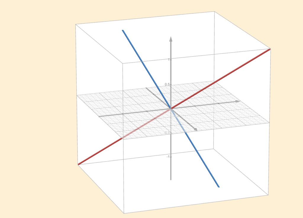
These are our orthogonal subspaces. No matter which \(\mathbf{u} \in U_1\)​ or \(\mathbf{v} \in U_2\)​​ you choose, they will be perpendicular to each other. However, we also know that \(\text{dim}(\mathbb{R}^3)=3\). Each of these subspaces has dimension \(1\), since a single nonzero vector, together with all its scalar multiples, spans the entire subspace. This means one dimension is missing, because \(3−1−1=1\).

If two subspaces are orthogonal to each other and their dimensions add up to the dimension of the whole space, then we call one the orthogonal complement of the other. One subspace “completes” the other by being perpendicular to it and filling the rest of the space. In the example above, the two lines are perpendicular, but neither is the orthogonal complement of the other.

If our vector space is \(\mathbb{R}^3\) and our subspace is a one-dimensional line, then its orthogonal complement must have dimension \(2\) and be orthogonal to that line. It fills the remaining part of the space, in this case, it is a plane in \(\mathbb{R}^3\). Specifically, in \(\mathbb{R}^3\), orthogonal complements can only have dimensions \(2\) and \(1\), or \(3\) and \(0\).

If you have a vector \(\mathbf{v}\) and you know that it is orthogonal to some vector in the first subspace, then it must lie in the second subspace, and vice versa. Formally:

We have some important properties that are worth remembering:

• If \(U\) is a subset of \(V\), then \(U^{\perp}\) is a subspace of \(V\).
• \(\{0\}^{\perp} = V\).
• \(V^{\perp} = \{0\}\).
• If \(U\) is a subset of \(V\), then \(U \cap U^{\perp} \subseteq \{0\}\).
• If \(U_1\) and \(U_2\) are subsets of \(V\) and \(U_1 \subseteq U_2\), then \(U_2^{\perp} \subseteq U_1^{\perp}\).

It is also worth highlighting that if you take the orthogonal complement of the orthogonal complement, that is, \((U^{\perp})^{\perp} = U\), you return to the original space. (If \(U\) is finite-dimensional.)

Here are also the formal definitions, which basically say that the orthogonal complement fills the rest of the space:

Finally, the following definition says that if your orthogonal complement is the zero vector, then your subspace is the whole vector space \(V\), and vice versa.

The Four Fundamental Subspaces

Recall that every linear transformation \(T\) naturally comes with two important subspaces. One is the null space, made up of all input vectors that \(T\) sends to zero. The other is the range (or column space in matrix terms), which consists of all vectors that \(T\) can actually produce.

From the previous chapter, we also know that every linear transformation has an associated adjoint \(T^*\) (In the context of inner product spaces, as assumed here). Just like \(T\), the adjoint has its own null space and its own range. Altogether, this gives us four subspaces tied to a single linear transformation. Since these subspaces come automatically, no extra choices or assumptions required, we call them the four fundamental subspaces. Think of it like one of those buy-two-get-two deals. The word “fundamental” simply reflects the fact that they are always there.

These four subspaces don’t all live in the same vector space. The null space of \(T\) lives in the input space \(V\) (or \(\mathbb{R}^n\) in matrix language), while the range of \(T\) lives in the output space \(W\) (or \(\mathbb{R}^m\)). The adjoint reverses direction: if \(T:V \rightarrow W\), then \(T^*:W \rightarrow V\). As a result, the null space of \(T^*\) lives in \(W\), and the range of \(T^*\) lives back in \(V\).

The truly interesting part is that these subspaces come in orthogonal complement pairs. To get a clearer picture of how all these pieces fit together, we’ll look at each vector space on its own.

Input Vector Space \(\mathbb{R}^n\)

This space includes two separate subspaces, where one is the orthogonal complement of the other. More specifically, we have the null space of \(T\) and the range of \(T^*\). In previous chapters, I hinted at the idea of a row space. This is where it comes from.

Just as we gave the range of \(T\) the name column space using its matrix representation, we can do the same for \(T^*\). However, since \(T^*\) is represented by \(A^{\top}\), the columns of \(A^{\top}\) are simply the rows of \(A\). So instead of calling it the column space of \(A^{\top}\), we usually call it the row space, although \(\text{Col}(A^{\top})\) is also very common.

If our input space is three-dimensional, meaning \(\text{dim}(V)=3\), and the null space is one-dimensional, then its orthogonal complement, namely the row space, must be two-dimensional. Recall that we call the dimension of this space the rank, and also remember that the row rank equals the column rank. This connection will prove to be extremely useful.

Gilbert Strang’s figure below illustrates the relationship between the row space and the null space quite well.

These two subspaces only share the zero vector, as indicated by the arrow in the figure. Notice also the right-angle symbol, which represents orthogonality. This is the most general case. However, remember that if \(T\) is invertible, the null space contains only the zero vector. In that situation, the null-space square in the figure essentially disappears, and everything lies in the row space, the row space fills the entire input space.

We can also have the opposite extreme, where the entire space is the null space. This occurs only for the zero transformation (or its matrix representation, the zero matrix). In that case, the row-space square disappears instead.

This figure is cool and all, but what does this actually look like in practice? Say no more.

Example

Consider the following matrix:

\(A = \begin{bmatrix} 1 & 1 \\ 2 & 2\end{bmatrix}\)

It shouldn’t be hard to see that this matrix is not invertible: the first and second columns are literally the same. This means we lose information. That lost information is hiding in the null space, which tells us that the null space is larger than just the zero vector. Let’s illustrate this.

The columns of \(A^{\top}\) (rows of \(A\)) both lie along the vector \((1,1)\), which means the row space is simply the span of that vector. To find the null space, we need a solution to \(A\textbf{x}=\mathbf{0}\). Normally, you would use row-reduced echelon form, but that would be overkill here. Instead, notice that if we take the first column of \(A\) and subtract the second, we get the zero vector. This means that the vector \((1,−1)\) lies in the null space. (Any scalar multiple of this vector would also satisfy the equation.)

Drawing these subspaces gives:

---

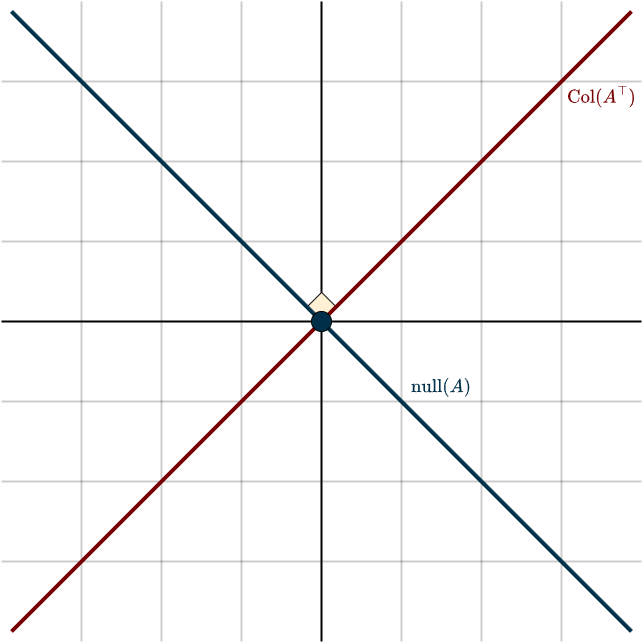
Using the matrix perspective, we can clearly see that the row space is orthogonal to the null space. Consider the equation

\(A\mathbf{x} = \mathbf{0}\)

Writing this out explicitly gives

\(A\mathbf{x} = \begin{bmatrix} \text{row } 1 \\ \vdots \\ \text{row } m \end{bmatrix} \mathbf{x} = \begin{bmatrix} 0 \\ \vdots \\ 0 \end{bmatrix}\)

We can view matrix–vector multiplication through the lens of the dot product. In this interpretation, the first entry of the resulting vector is the dot product of the first row of \(A\) with the vector \(\mathbf{x}\). This gives

\((\text{row } 1) \cdot \mathbf{x} = \mathbf{0}\)

\(\vdots\)

\((\text{row } m) \cdot \mathbf{x} = \mathbf{0}\)

This tells us that any vector \(\mathbf{x}\) satisfying \(A\mathbf{x} = \mathbf{0}\), that is, any vector in the null space, is orthogonal to every row vector of \(A\).

Output Vector Space \(\mathbb{R}^m\)

Similar to the input space, the output space also contains two subspaces that are orthogonal complements of each other. These are the column space of \(A\) (range of \(T\)) and the null space of \(T^*\). Since we already use the term null space for \(T\) itself, we’ll call this second one the left null space. You’ll also often see it referred to as the null space of \(A^{\top}\).

The same “filling up the space” idea applies here. For example, if the output space is three-dimensional and the column space is one-dimensional, then the left null space must account for the remaining two dimensions. Just like before, we can relate the dimensions of the column space and the row space through the rank of the matrix, since column rank and row rank are always equal. Using a similar diagram as earlier, this gives us the following picture:

Again, if the transformation is invertible, meaning no information is lost, then the left null space contains only the zero vector. In the figure, this makes the left-null-space square disappear entirely, leaving the column space to cover the whole output space. On the other extreme, if we have the zero transformation (or the zero matrix), the column space vanishes instead.

Example

Consider the matrix

\(A = \begin{bmatrix} 1 & 2 \\ 3 & 4 \\ 3 & 6 \end{bmatrix}\)

We can immediately see that \(A\) isn’t invertible because it’s not square. Still, its columns are linearly independent, so the column space has dimension \(2\). In other words, the column space is a two-dimensional plane in \(\mathbb{R}^3\). To get a better sense of the left nullspace, it’s easiest to look at the transpose of \(A\):

\(A^{\top} = \begin{bmatrix} 1 & 3 & 3 \\ 2 & 4 & 6 \end{bmatrix}\)

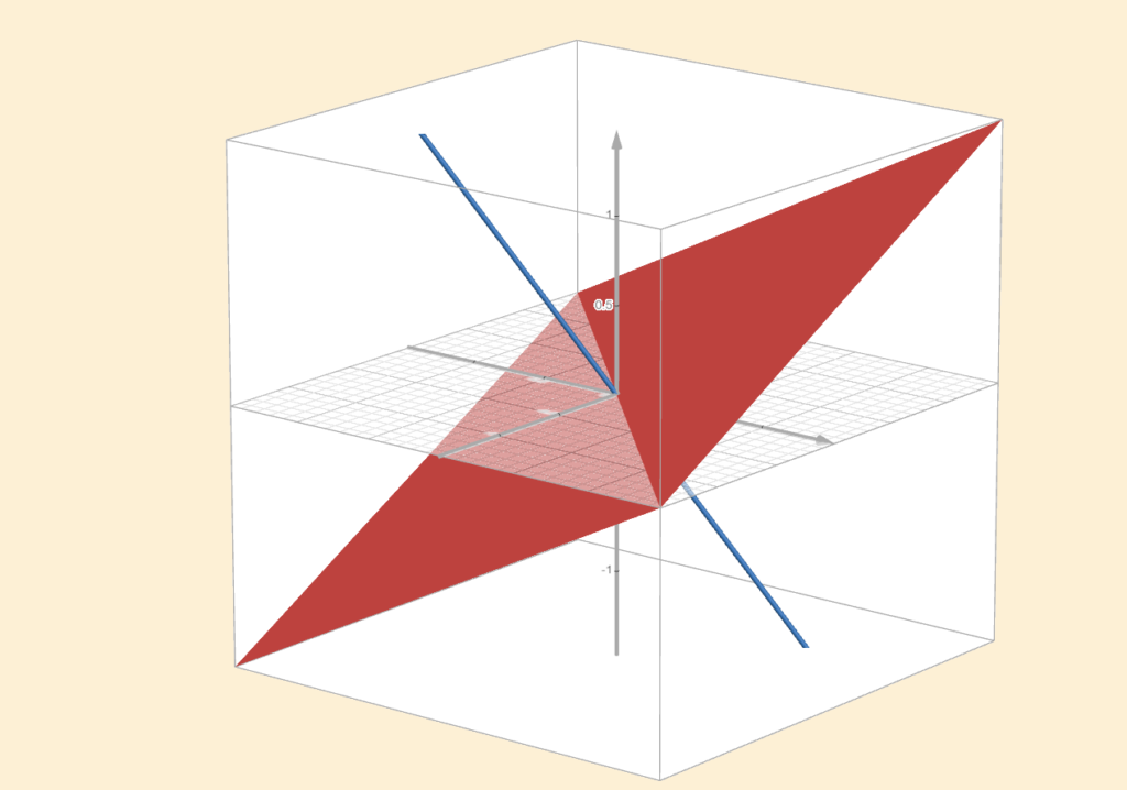
The left null space, the orthogonal complement of the column space, must be one-dimensional. In other words, there is a single direction (along with all its scalar multiples) that spans this space. Again, we are looking for a linear combination of the columns of \(A^{\top}\) that gives the zero vector. If you look closely, you can see that the third column is three times the first one, so the vector \((−3,0,1)\) gives the desired combination. The figure below shows how these subspaces look.

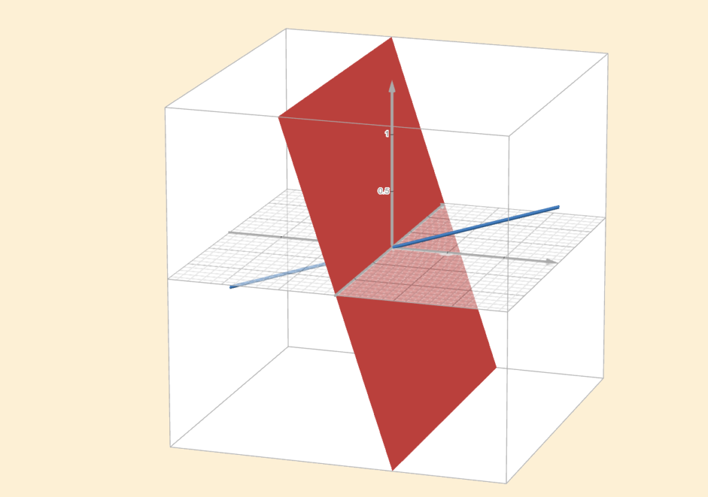
The plane highlighted in red represents the column space, while the blue line represents the left null space.

If you are wondering why we call this the left null space, here is the reason. Recall that the columns of \(A^{\top}\) are the rows of \(A\). So if a vector \(\mathbf{y}\) forms a combination of the columns of \(A^{\top}\) that gives zero, then the same combination acting on the rows of \(A\) will also give zero. In algebraic terms,

\((A^{\top}\mathbf{y})^{\top} = \mathbf{0}^{\top} \hspace{0.5cm} \rightarrow \hspace{0.5cm} \mathbf{y}^{\top} A = \mathbf{0}\)

Since \(\mathbf{y}\) acts on \(A\) from the left to produce the zero row, we call this the left null space.

The matrix perspective also shows again why the left null space is orthogonal to the column space. Starting from

\(A^{\top} \mathbf{y} = \mathbf{0}\)

we see that each column of \(A\) (equivalently, each row of \(A^{\top}\)) has zero dot product with a vector from the left null space. This means they are orthogonal.

---

We’ve now seen what each orthogonal complement pair looks like in its respective vector space. Next, we can bring them together to form the complete picture.

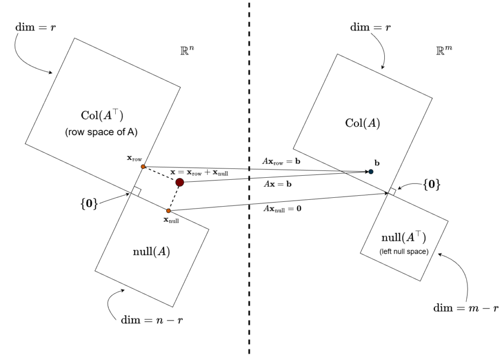
There’s a lot going on here, so let’s slow down and unpack it. Start with the basics: we have an input space \(\mathbb{R}^n\) and an output space \(\mathbb{R}^m\). Each of these spaces contains two subspaces that come in orthogonal pairs. The dimensions already hint at this structure.

The number \(r\) is the rank, the dimension of the column space. And since column rank equals row rank, the row space also has dimension \(r\). The dimensions of the remaining two subspaces then follow automatically from the orthogonal complement property.

Now here’s an important point that’s easy to miss. These orthogonal pairs do not split the input or output spaces in an “either–or” sense. A vector isn’t forced to live strictly in one subspace or the other. Remember the idea of adding subspaces: a subspace plus its orthogonal complement gives the entire space. That means a vector can live in their sum.

Look at the vector \(\mathbf{x}\) in the figure. It lives in the input space, but it’s not purely in the row space or purely in the null space. What the orthogonal complement gives us is a clean way to split \(\mathbf{x}\) into two pieces: one part in the row space and one part in the null space. The vector \(\mathbf{x}\) itself is the sum of those two components, and that sum is the whole input space.

This idea of decomposing a vector into pieces from different subspaces isn’t new, we’ve already seen it earlier when talking about subspaces. What is new here is how this split works: the pieces are perpendicular. Because the row space and null space meet at right angles, changing one component doesn’t affect the other. You can slide the vector along the null space direction without touching the row space component, and vice versa. The contributions from each subspace don’t interfere with each other. That’s the real power of orthogonality.

Now follow what happens under the transformation. The row space component of \(\mathbf{x}\) gets mapped to the right-hand side vector \(\mathbf{b}\), while the null space component gets sent straight to the zero vector in the output space. The dotted line in the middle of the diagram acts as a bridge, marking the passage from the input world to the output world.

Here’s where things get interesting. The mapping from \(\mathbf{x}\) to \(\mathbf{b}\) is generally not invertible. The null space is the culprit: different vectors can collapse to the same output, so information is lost and we can’t undo the mapping. But once we split \(\mathbf{x}\) into its row space and null space parts, something changes. We can ignore the evil null space component, the part that gets wiped out anyway, and focus entirely on the row space component. That piece is invertible.

This is the core idea behind the pseudoinverse. When an exact inverse doesn’t exist, we don’t give up, we look for the best possible solution by keeping the meaningful part and discarding the rest. We’ll dig into this idea properly soon.

Summary

• Two subspaces are orthogonal if every vector in the first subspace is orthogonal to every vector in the second.
• Two subspaces are orthogonal complements if they are orthogonal and together span the entire space. In other words, one subspace “fills in” exactly the directions missing from the other.
• Every linear transformation has a null space and a range (column space). In inner product spaces, each linear transformation also has an adjoint, which comes with its own null space and range. These are called the left null space and the row space, respectively.
• In the input space, the orthogonal complement pair is: null space and row space
• In the output space, the orthogonal complement pair is: left null space and column space
• Because the input space splits into these two orthogonal subspaces, any input vector can be decomposed uniquely into two components: one in the null space and one in the row space. The null space component is sent to zero by the transformation, while the row space component is mapped to a vector in the output space.