Orthogonal Matrices and Householder QR
How can we extract a stable orthogonal structure from any matrix?
An orthonormal basis makes computations fast, stable, and simple. If the columns of a matrix are orthonormal, we denote it by \(Q\). Such a matrix preserves the inner product. In general, the adjoint and the inverse of a linear transformation are different, except in this special case where they coincide. Not every matrix \(A\) has orthogonal columns. But we can extract orthogonality from it by decomposing it as \(A = QR\). The Householder algorithm gives us the most stable way to compute this decomposition.
Orthogonal Matrix
Recall that a list of vectors is orthonormal if every vector is orthogonal to the others and each has unit length. We’ve already seen how powerful an orthonormal basis can be, it makes calculations cleaner and often dramatically simpler. But what happens if the columns of a matrix are orthonormal? In the previous chapter, something interesting happened:
\(A^{\top}A = I\)
It almost felt like magic. Why should that be true?
Let’s look carefully at what \(A^{\top}A\) actually does when the columns of \(A\) are orthonormal.
\(A^{\top}A = \begin{bmatrix} \text{— } \mathbf{a}_1^{\top} \text{ —} \\ \text{— } \mathbf{a}_2^{\top} \text{ —} \\ \text{— } \mathbf{a}_3^{\top} \text{ —}\end{bmatrix} \begin{bmatrix} | & | & | \\ \mathbf{a}_1 & \mathbf{a}_2 & \mathbf{a}_3\\ | & | & | \end{bmatrix} = \begin{bmatrix} \mathbf{a}^{\top}_1\mathbf{a}_1 & \mathbf{a}^{\top}_1 \mathbf{a}_2 & \mathbf{a}^{\top}_1 \mathbf{a}_3 \\ \mathbf{a}^{\top}_2\mathbf{a}_1 & \mathbf{a}^{\top}_2\mathbf{a}_2 & \mathbf{a}^{\top}_2\mathbf{a}_3 \\ \mathbf{a}^{\top}_3\mathbf{a}_1 & \mathbf{a}^{\top}_3\mathbf{a}_2 & \mathbf{a}^{\top}_3\mathbf{a}_3\end{bmatrix} = \begin{bmatrix} 1 & 0 & 0\\ 0 & 1 & 0 \\ 0 & 0 & 1 \end{bmatrix} = I\)
Each entry is just an inner product between two columns. Now recall:
- Different columns are orthogonal → their inner product is 0.
- Each column has unit length → its inner product with itself is 1.
So every off-diagonal entry becomes \(0\), and every diagonal entry becomes \(1\).
We usually denote a matrix with orthonormal columns by \(Q\). Important: \(Q\) does not need to be square. Just like \(A\) before, it can be rectangular. The only requirement is that its columns are orthonormal. The linear transformation behind such a matrix is called an isometry. Formally:
A linear map \(S \in \mathcal{L}(V, W)\) is called an isometry if
\(||S\mathbf{v}|| = ||\mathbf{v}||\)
for every \(\mathbf{v} \in V\). In other words, a linear map is an isometry if it preserves norms.
(And don’t mix up this letter \(S\) with the \(S\) we sometimes use for symmetric matrices. Same letter, different role.)
The word isometry comes from Greek: isos means equal and metron means measure. So it literally means “equal measure.” The more you know…
Now, a general linear transformation \(T\) distorts geometry: Some directions get stretched. Some get compressed. Some might even collapse completely. Angles change. Distances change. That’s why we previously needed \((A^{\top}A)^{-1}\) to “correct” measurements. But with a matrix \(Q\) whose columns are orthonormal, this distortion does not happen. Yes, if \(Q\) is rectangular, you may lose some directions (because the target space might be lower-dimensional). But the directions that remain are still perfectly orthonormal. The transformation moves vectors, but it does not mess with Euclidean geometry.
You can see this directly:
\(||Q\mathbf{x}|| = (Q\mathbf{x})^{\top} = \mathbf{x}^{\top}Q^{\top}Q\mathbf{x} = \mathbf{x}^{\top} I \mathbf{x} = \mathbf{x}^{\top} \mathbf{x} = ||\mathbf{x}|| \)
\(\langle Q\mathbf{x}, Q\mathbf{y} \rangle = (Q\mathbf{x})^{\top}(Q\mathbf{y}) = \mathbf{x}^{\top}Q^{\top}Q\mathbf{y} = \mathbf{x}^{\top} I \mathbf{y} = \mathbf{x}^{\top}\mathbf{y} = \langle \mathbf{x}, \mathbf{y} \rangle\)
\(Q\) preserves lengths and angles. You must appreciate the power of this result. Imagine you’re training a machine learning model where parameters form a matrix. Suppose each multiplication stretches vectors just a tiny bit. Then at every layer, the representation (our numbers) grows slightly. After many layers, your numbers explode. Numerical instability becomes a serious problem. This does not happen with \(Q\). Since \(Q\) preserves lengths, it cannot gradually inflate your representations. That’s an enormous stability advantage.
If \(Q\) is square, you get an extra bonus. Since it’s square, we can multiply on both sides and obtain
\(Q^{\top}Q = QQ^{\top}= I\)
That looks suspiciously like the definition of an inverse. And you’d be absolutely right:
\(Q^{-1} = Q^{\top}\)
A square matrix with orthonormal columns is called an orthogonal matrix. I didn’t choose the naming. It is slightly confusing that only the square case gets a special name, while the rectangular one is just called “a matrix with orthonormal columns.” But that’s the convention. The underlying linear transformation in the square case is called unitary. Formally:
An operator \(S \in \mathcal{L}(V)\) is called unitary if \(S\) is an invertible isometry.
Here is the reason why this is so powerful: Computing a matrix inverse is usually a pain. Here, you just transpose, switch rows and columns, and you’re done.
Why is the Adjoint suddenly the Inverse?
How can “the thing that changes measurements” suddenly become the inverse of a linear transformation? Let’s first clarify the difference between the inverse and the adjoint.
The inverse of a linear transformation exists independently of any basis, any coordinate system, and it does not require an inner product.
If \(T\) moves vectors in a certain way, then \(T^{−1}\) simply undoes that movement, if that’s possible. The adjoint, on the other hand, conceptually answers a different question: How can we adjust things so that the inner product behaves the same before and after applying the linear transformation? This is about preserving measurements, and specifically about how covectors (or linear functionals) must transform.
And this is the key difference:
- The inverse is purely about undoing a transformation.
- The adjoint depends on the inner product.
Remember, the adjoint is essentially the dual map with extra steps. We:
- Turn vectors in \(W\) into covectors in \(W′\) (using the Riesz map),
- Apply the dual map to move to \(V′\),
- Convert back into vectors in \(V\).
The dual map itself does not care about the inner product. But the identification between vectors and covectors, the Riesz map, relies entirely on the inner product. Without it, the adjoint wouldn’t even be defined in this way. Now here’s the key question: Why do the adjoint and the inverse become the same when \(T\) preserves the inner product?
By “preserves the inner product,” we mean:
\(\langle T\mathbf{x}, T\mathbf{y} \rangle = \langle \mathbf{x}, \mathbf{y} \rangle\)
In other words, the dot product is the same before and after applying \(T\). This means: Angles don’t change. Lengths don’t change. Nothing stretches or shrinks. Geometrically, this corresponds to a rigid motion. Imagine holding a book in your room. If you rotate it, it’s still the same book, not bigger, not smaller, not stretched. Just rotated. Now imagine holding it in front of a mirror. The reflection is still the same book. Distances and angles are preserved. That’s exactly what orthogonal transformations do. They correspond to pure rotations or reflections across some subspace. If you imagine the coordinate grid of the input space \(V\), the grid after transformation looks exactly the same, just rotated or reflected. No distortion.
So why are they equal in this case? Here’s the core idea. Because \(T\) is invertible (unitaries must be), we can rewrite
\(\langle T\mathbf{x}, \mathbf{y} \rangle = \langle T\mathbf{x}, I\mathbf{y} \rangle = \langle T\mathbf{x}, T(T^{-1}\mathbf{y}) \rangle\)
Now apply the isometry property
\(\langle T\mathbf{x}, T(T^{-1}\mathbf{y}) \rangle = \langle \mathbf{x}, T^{-1}\mathbf{y} \rangle\)
This means that
\(\langle T\mathbf{x}, \mathbf{y} \rangle = \langle \mathbf{x}, T^{-1}\mathbf{y} \rangle\)
But compare this with the defining equation of the adjoint
\(\langle T\mathbf{x}, \mathbf{y} \rangle = \langle \mathbf{x}, T^{*}\mathbf{y} \rangle\)
Since both expressions must hold for all vectors \(\mathbf{x}\), we conclude
\(T^*\mathbf{y} = T^{-1}\mathbf{y}\)
But this also holds for all \(\mathbf{y}\)
\(T^*= T^{-1}\)
Because \(T\) does not distort anything, the only way to move back consistently is to literally undo it. So in this special case: The inverse undoes the geometric motion. The adjoint undoes the measurement change. But since there was no distortion to compensate for, both operations become the same.
Let’s make this more concrete with an example.
Example
Consider the following figure.
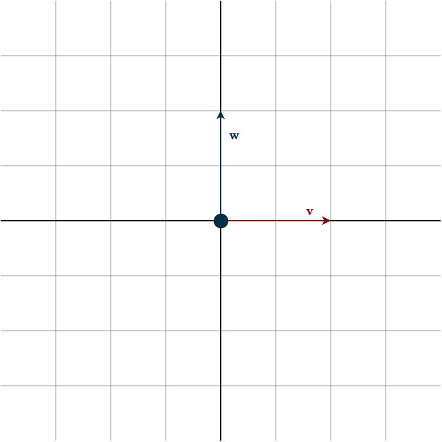
Suppose we want to measure the “up” component of a vector \(\mathbf{v}\), in other words, how strongly it points in the upward direction. To do that, we introduce another vector \(\mathbf{w}\) that points exactly upward. From the projection chapter, we know that the dot product between two vectors tells us how much one vector points in the direction of the other. Conceptually, we’re projecting one vector onto the other. So if we take the dot product between \(\mathbf{w}\) and \(\mathbf{v}\), we directly measure how much “up” there is in \(\mathbf{v}\). Remember that once we fix \(\mathbf{w}\) and use it inside a dot product, it becomes a linear functional, a covector, that measures other vectors. In this case.
\(\mathbf{w}^{\top} \mathbf{v} = \begin{bmatrix} 0 & 1\end{bmatrix} \begin{bmatrix} 1 \\ 0\end{bmatrix} = 0\)
This shouldn’t be surprising, since the vectors are perpendicular. There’s no “up” component in \(\mathbf{v}\). Now let’s rotate \(\mathbf{v}\) by 90° clockwise. This transformation is described by the matrix
\(Q = \begin{bmatrix} 0 & 1 \\ -1 & 0\end{bmatrix}\)
Applying it to \(\mathbf{v}\) gives:
\(Q\mathbf{v} = \begin{bmatrix} 0 & 1 \\ -1 & 0\end{bmatrix} \begin{bmatrix} 1 \\ 0\end{bmatrix} = \begin{bmatrix} 0 \\ -1 \end{bmatrix}\)
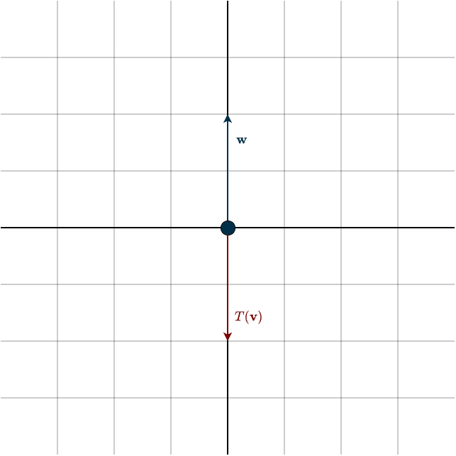
Now if we measure the “up” direction again, we get:
\(\mathbf{w}^{\top} T(\mathbf{v}) = \begin{bmatrix} 0 & 1\end{bmatrix} \begin{bmatrix} 0 \\ -1 \end{bmatrix} = -1\)
So now the vector lies completely in the vertical direction, just pointing downward instead of upward. At this point, we’ve answered our question. But notice what we had to do:
- Measure.
- Apply the transformation.
- Measure again.
If we want to repeat this for many vectors, this quickly becomes tedious. Enter the adjoint: instead of transforming \(\mathbf{v}\), what if we leave \(\mathbf{v}\) fixed and transform \(\mathbf{w}\), the measurement vector, instead? There’s one crucial requirement: the final measurement must stay the same. In this case, it must still produce \(−1\). There is exactly one way to transform \(\mathbf{w}\) so that this happens.
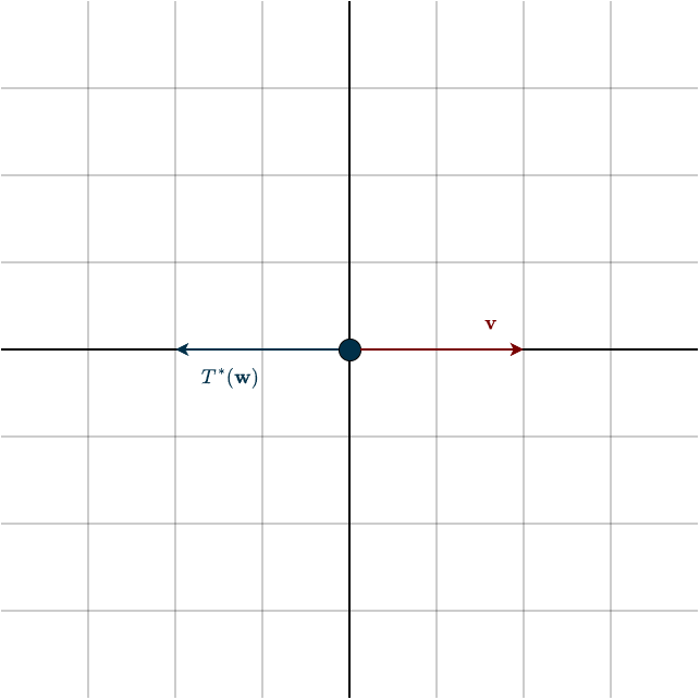
What happened? The adjoint rotated \(\mathbf{w}\) by 90° counterclockwise. That produces the same measurement, without ever touching \(\mathbf{v}\). This is the real power of the adjoint. Instead of transforming every vector and then measuring, we transform the measurement itself. And we don’t just adjust one question, we adjust all possible measurements at once. Just as \(T\) transforms every vector it acts on, the adjoint \(T^∗\) transforms every covector it acts on. And since we can move between vectors and covectors using the inner product, this becomes especially elegant: This counterclockwise rotation is exactly the same one performed by the inverse.
To see why the adjoint is generally different than the inverse, consider another setup. Take the same vector \(\mathbf{v}\), but now suppose we only want to measure its length, not a specific direction. And instead of rotating, we stretch space by a factor of \(2\) in the first coordinate direction. So vectors pointing in that direction become twice as long. The inverse transformation would simply shrink everything back to its original size. But the adjoint behaves differently. Since it must preserve the measurement relationship, it adjusts the measurement vector instead. In this case, it stretches the measurement by a factor of \(2\) rather than undoing the transformation.
So the inverse undoes what \(T\) does to vectors. The adjoint adjusts measurements to keep inner products consistent. These are fundamentally different goals. And that’s why, in general \(T \neq T^*\).
A = QR via Householder
Orthogonal matrices have clearly been the heroes so far. They are numerically stable and computationally efficient. So why don’t we just use them everywhere? The issue is that the matrix \(A\) we start with is usually not orthogonal. The problem we are solving determines how \(A\) looks, and in general it does not magically come with orthogonal columns. That means we cannot directly benefit from all those amazing properties orthogonal matrices give us.
But this is not bad news. Just like we decomposed a matrix into \(LU\), we can also decompose \(A\) into
\(A = QR\)
where \(Q\) is orthogonal and \(R\) is upper triangular. Once we have this decomposition, we can reuse it many times. The whole point of this is to transform the columns of \(A\) into an orthonormal basis. The columns of \(A\) may be linearly dependent, and \(A\) itself may be rectangular, but our aim is to extract the best possible basis from its column space.
Classically, the Gram–Schmidt algorithm is used to transform \(A\) into \(QR\). It is conceptually simple and elegant. Under the hood, it works using projections:
- Take one column of \(A\)
- Project it onto the previous columns
- Subtract the projected part
- What remains is perpendicular
Simple and beautiful. But this exact projection step is also its weakness. If the columns of \(A\) are very close to being linearly dependent (but not exactly dependent), numerical errors can become large. Floating-point rounding errors accumulate, and in practice the resulting \(Q\) is often not perfectly orthogonal. It is therefore numerically unstable (especially the classical version). In addition, it is more sequential in nature and harder to optimize for modern hardware. In modern applications, matrices are very large. Efficiency and stability are not optional, they are essential.
This is why we use the Householder approach to compute \(A=QR\). It is numerically stable, produces highly orthogonal \(Q\), more robust for ill-conditioned matrices and well optimized for modern hardware. Gram–Schmidt is excellent for teaching the idea of orthogonalization. But in practice, Householder reflections are usually the better tool.
To really understand how the Householder algorithm works, we need to take a closer look at reflections. A reflection is simply mirroring an object across some kind of barrier or divider. Imagine holding a book in front of a mirror. The mirror is the barrier, and the image you see is the reflected object. In linear algebra, we reflect a vector across a subspace.
The important question is: how can we construct a linear transformation, and therefore a matrix, that reflects every vector across a given subspace?
First, we need to describe the subspace we are reflecting across. One option would be to use a spanning set. But that quickly becomes awkward. If the dimension of the subspace changes, the spanning set changes as well. The algorithm would need to adapt each time. And working with many vectors is generally inconvenient. The fewer objects we have to track, the better. There is a much simpler idea. Recall the concept of orthogonal complements. Instead of directly describing the subspace we reflect across, we describe the direction perpendicular to it. Even better, we make that perpendicular space one-dimensional. That means we only need a single vector. Let us call it \(\mathbf{u}\).
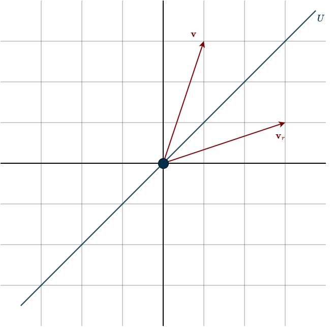
To simplify the calculations, we assume \(\mathbf{u}\) is a unit vector, so \(\mathbf{u}^{\top}\mathbf{u} = 1\). No matter whether the subspace we reflect across has dimension \(2\) or \(10\), we only need to keep track of this one vector \(\mathbf{u}\). That is what makes the method so clean. Look at the setup below.
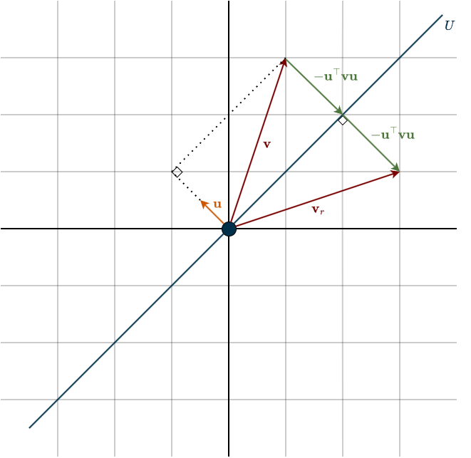
Now suppose we want to reflect a vector \(\mathbf{v}\). We begin by taking the projection of \(\mathbf{v}\) onto \(\mathbf{u}\). The projection formula is
$$\frac{\mathbf{u}^{\top}\mathbf{v}}{\mathbf{u}^{\top} \mathbf{u}}\mathbf{u}$$
Since \(\mathbf{u}\) is a unit vector, this simplifies to
\((\mathbf{u}^{\top}\mathbf{v})\mathbf{u}\)
Starting from \(\mathbf{v}\), and then subtracting twice its projected component, gives exactly the reflected vector
\(\mathbf{v}_r = \mathbf{v} \; – \; 2 (\mathbf{u}^{\top}\mathbf{v})\mathbf{u}\)
Notice that \(\mathbf{u}^{\top}\mathbf{v}\) is a scalar. Scalar multiplication commutes with vectors, so we can rewrite this as
\(\mathbf{v}_r = \mathbf{v} \; – \; 2 \mathbf{u} (\mathbf{u}^{\top}\mathbf{v})\)
Now place the parentheses carefully
\(\mathbf{v}_r = \mathbf{v} \; – \; 2 (\mathbf{u} \mathbf{u}^{\top})\mathbf{v}\)
Recall that the expression \(\mathbf{u}\mathbf{u}^{\top}\) is a matrix. That is already a big step forward. The only thing left is to factor out \(\mathbf{v}\). Unlike with numbers, we cannot simply replace it by \(1\). Instead, we use the identity matrix \(I\), which plays the role of the multiplicative identity for matrices
\(\mathbf{v}_r = I\mathbf{v} \; – \; 2 (\mathbf{u} \mathbf{u}^{\top})\mathbf{v} = (I \; – \; 2 \mathbf{u} \mathbf{u}^{\top}) \mathbf{v}\)
This means that the reflection matrix is
\(H = I \; – \; 2 \mathbf{u} \mathbf{u}^{\top}\)
Pay attention to the \(H\). As you can see, this transformation is unitary, that is, it is represented by an orthogonal matrix. Even more remarkably, the matrix is also symmetric
\(H^{\top} = (I \; – \; 2 \mathbf{u} \mathbf{u}^{\top})^{\top} = I^{\top} \; – \; 2 (\mathbf{u} \mathbf{u}^{\top})^{\top} = I \; – \; 2 (\mathbf{u}^{\top})^{\top} \mathbf{u}^{\top} = I \; – \; 2 \mathbf{u} \mathbf{u}^{\top} = H\)
Which means
\(H = H^{\top} = H^{-1}\)
So the matrix is its own inverse, which kind of makes sense. If you mirror something twice, you end up right back where you started. This reflection matrix is the fundamental building block of the Householder QR algorithm.
Now how does the actual algorithm work? The goal is to transform \(A\) into an upper triangular matrix \(R\). In other words, we want to eliminate all entries below the diagonal. Let’s focus on the first step. We are looking for a matrix \(H_1\) such that, when multiplied on the left of \(A\), it zeros out all entries below \(a_{11}\):
\(H_1 A = H_1 \begin{bmatrix} a_{11} & a_{12} & a_{13} \\ a_{21} & a_{22} & a_{23} \\ a_{31} & a_{32} & a_{33} \end{bmatrix} = \begin{bmatrix} a_{11} & a_{12} & a_{13} \\ 0 & a_{22} & a_{23} \\ 0 & a_{32} & a_{33} \end{bmatrix}\)
At first, you might think: why not just use Gaussian elimination like in LU decomposition? The issue is that elimination matrices are not orthogonal, and here we specifically need an orthogonal transformation. Notice something important: after this transformation, the first column looks like a scaled version of the first standard basis vector \(\mathbf{e}_1\). All entries except the first are zero. So what we really want is a transformation that converts the first column of \(A\), call it \(\mathbf{a}_1\), into a multiple of \(\mathbf{e}_1\).
We can think of this geometrically. Instead of asking, What does a vector look like after reflecting across a given subspace?, we ask the reverse question: Across which subspace should we reflect \(\mathbf{a}_1\) so that it becomes aligned with \(\mathbf{e}_1\)? We are searching for the right “mirror” so that reflecting \(\mathbf{a}_1\) across it produces a vector in the direction of \(\mathbf{e}_1\).
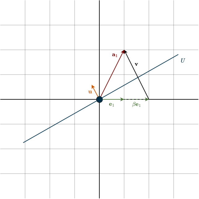
If you look closely at the figure, you’ll notice that \(\mathbf{v}\) and \(\mathbf{u}\) are parallel, they point in the same direction. In fact, they’re essentially the same vector, except that one is just a scaled version of the other. That is, \(\mathbf{v}\) is simply some scalar multiple of \(\mathbf{u}\). Finding this vector \(\mathbf{v}\) is the key step. Once we have \(\mathbf{v}\), we can determine \(\mathbf{u}\), and with \(\mathbf{u}\) we can describe the subspace. From that subspace, we can then identify the transformation we’re looking for. Now, \(\mathbf{v}\) is nothing more than
\(\mathbf{v} = \mathbf{a}_1 \; – \; \beta \mathbf{e}_1\)
Because the reflection is represented by an orthogonal matrix, it preserves lengths. That means the reflected vector must have the same norm as \(\mathbf{a}_1\). Since \(\mathbf{e}_1\) has length \(1\), we must have
\(|\beta| = ||\mathbf{a}_1||\)
Notice the absolute value. \(\beta\) could be positive or negative. Both choices give a vector aligned with \(\mathbf{e}_1\), just in opposite directions. Below is the example of the negative case.
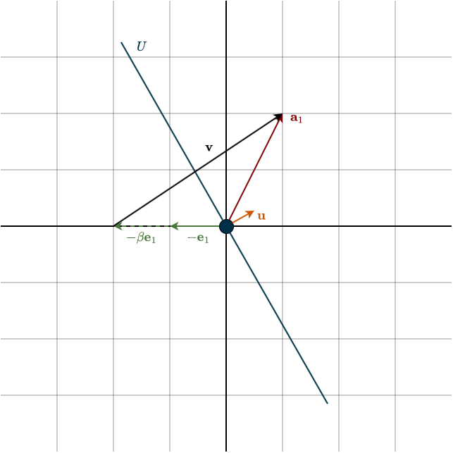
So which sign should we choose? Let’s write \(\mathbf{v}\) more explicitly:
\(\mathbf{v} = \mathbf{a}_1 \; – \; \beta \mathbf{e}_1 = \begin{bmatrix} a_{11} \\ \vdots \\ a_{1m} \end{bmatrix} \; – \; ||\mathbf{a}_1||\begin{bmatrix} 1 \\ \vdots \\ 0 \end{bmatrix} = \begin{bmatrix} a_{11} \\ \vdots \\ a_{1m} \end{bmatrix} \; – \; \begin{bmatrix} ||\mathbf{a}_1|| \\ \vdots \\ 0 \end{bmatrix}\)
Now suppose most of the “weight” (i.e., magnitude) of \(\mathbf{a}_1\) lies in its first coordinate. If the vector is already close to the \(\mathbf{e}_1\) direction, then \(a_{11}\) is very close to \(||\mathbf{a}_1||\). In that case, subtracting \(||\mathbf{a}_1||\) from \(a_{11}\) causes catastrophic cancellation: we subtract two nearly equal numbers and lose significant numerical precision, and that is a big no no.
Fortunately, we have freedom in choosing the sign of \(\beta\). The fix is simple:
\(\beta = -\text{sign}(a_{11})||\mathbf{a}_1||\)
where
\(\text{sign}(a_{11}) = \begin{cases} 1 & \text{if } a_{11} \geq 0, \\ -1 & \text{if } a_{11} < 0 \end{cases}\)
By choosing the opposite sign of \(a_{11}\), we avoid subtracting nearly equal numbers. Instead, we effectively add magnitudes, which is numerically stable.
So far we have \(\mathbf{v}\), which gives us the correct direction, but it is not yet a unit vector. We need to normalize it:
$$\mathbf{u} = \frac{\mathbf{v}}{||\mathbf{v}||}$$
The (Householder-) reflection matrix is then
\(H_1 = I \; – \; 2\mathbf{u}\mathbf{u^{\top}}\)
This is exactly the orthogonal transformation that maps the first column of \(A\) to a scaled version of \(\mathbf{e}_1\).
So, what about the remaining columns? We repeat the same idea, but now we focus only on the lower-right \((n − 1) \times (n − 1)\) submatrix. We leave the first column untouched, after all, we just worked hard to fix it. So we construct a new reflection \(H_2\) that acts only on that submatrix. Structurally, it looks like the identity matrix, except that its lower-right block is replaced by the new Householder matrix.
\(H_2 = \begin{bmatrix} 1 & 0 & \cdots & 0 \\ 0 & * & \cdots & * \\ \vdots & \vdots & \ddots & \vdots \\ 0 & * & \cdots & * \end{bmatrix}\)
Then we repeat again on the \((n − 2) \times (n − 2)\) submatrix, and so on. After all reflections are applied, we obtain:
\(H_3H_2H_1A = R\)
Now multiply both sides by the inverse of the reflection matrices (Remember that \(H = H^{\top} = H^{-1}\))
$$A = (H_3H_2H_1)^{-1}R \hspace{0.5cm} \Longleftrightarrow \hspace{0.5cm} A = (H_1)^{-1}(H_2)^{-1}(H_3)^{-1} R \hspace{0.5cm} \Longleftrightarrow \hspace{0.5cm} A = \underbrace{H_1H_2H_3}_{Q}R$$
I would like to point out that the product of orthogonal matrices is itself orthogonal. This result is also intuitively clear. If one geometry-preserving transformation is followed by another, then their composition (that is, performing one after the other as a single transformation) must also preserve geometry. For example, a 30° clockwise rotation followed by another 30° clockwise rotation is equivalent to a single 60° clockwise rotation, which is again an orthogonal transformation. We can therefore combine them into a single matrix \(Q\)
\(A = QR\)
And that’s the whole idea: we successively reflect columns of \(A\) onto standard basis vectors using orthogonal transformations, until what remains is an upper triangular matrix \(R\).
Now we understand how \(Q\) is constructed and what it represents. But what about \(R\)? We know it’s upper triangular, but what does it actually mean? What are its entries telling us? Start from the definition
\(A = QR \hspace{0.5cm} \Longleftrightarrow \hspace{0.5cm} R = Q^{-1}A \hspace{0.5cm} \Longleftrightarrow \hspace{0.5cm} R = Q^{\top}A\)
If we look at the case \(n=3\), then
\(R = \begin{bmatrix} \mathbf{q}_1^{\top} \mathbf{a}_1 & \mathbf{q}_1^{\top} \mathbf{a}_2 & \mathbf{q}_1^{\top} \mathbf{a}_3 \\ 0 & \mathbf{q}_2^{\top} \mathbf{a}_2 & \mathbf{q}_2^{\top} \mathbf{a}_3 \\ 0 & 0 & \mathbf{q}_3^{\top} \mathbf{a}_3\end{bmatrix}\)
where \(\mathbf{q}_i\) are the columns of \(Q\), and \(\mathbf{a}_i\) are the columns of \(A\). Now notice what’s happening. Because \(Q\) has orthonormal columns, each \(\mathbf{q}_i\) has unit length and is perpendicular to the others. That means \(\mathbf{q}_i^{\top}\mathbf{a}_j\) is the scalar projection of \(\mathbf{a}_j\) onto the direction \(\mathbf{q}_i\).
So every entry of \(R\) is a projection coefficient. Think back to the geometric picture of projections onto an orthonormal basis: a vector was decomposed into pieces, each piece lying along one orthonormal direction. The original vector was just the sum of those orthogonal components. That is exactly what’s happening here. Each column of \(R\) contains the coordinates of the corresponding column of \(A\), expressed in the orthonormal basis formed by \(Q\). For example, look at the first column of \(R\). Only the first entry is nonzero. That tells us that \(\mathbf{a}_1\) lies entirely in the direction of \(\mathbf{q}_1\). To reconstruct \(\mathbf{a}_1\), we only need that one projection coefficient
\(\mathbf{a}_1 = (\mathbf{q}^{\top}_1\mathbf{a}_1)\mathbf{q}_1\)
Now look at the second column. It has two nonzero entries. That tells us:
\(\mathbf{a}_2 = (\mathbf{q}^{\top}_1\mathbf{a}_2)\mathbf{q}_1 + (\mathbf{q}^{\top}_2\mathbf{a}_2)\mathbf{q}_2\)
So \(\mathbf{a}_2\) is split into two orthogonal pieces, one along \(\mathbf{q}_1\), one along \(\mathbf{q}_2\). Adding them gives the full vector back.
Put simply:
- \(Q\) builds an orthonormal basis for the column space of \(A\).
- \(R\) tells you how to reconstruct each original column from that basis.
You can think of \(QR\) as doing three things:
- Take a skewed basis \(\mathbf{a}_1, \mathbf{a}_2, \dots, \mathbf{a}_n\).
- Turn it into an orthonormal basis \(\mathbf{q}_1, \mathbf{q}_2, \dots, \mathbf{q}_n\), this is \(Q\).
- Record how to rebuild the original vectors from the new orthonormal ones, that record is \(R\).
So QR isn’t just a factorization. It’s a change of basis, plus the exact instructions for reversing it.
QR Implementation
Now it’s time to actually implement the algorithm. We’ll go step by step.
First, we define a function with a clear name that takes two parameters.
- The matrix \(A\).
This can be any matrix. It does not need to be square, invertible, or even have full column rank. Full column rank only becomes important later if we want to solve systems efficiently, either directly or via least squares to compute the best possible fit. But for computing the QR decomposition itself, none of those assumptions are required. - A flag called
"mode".
This allows us to switch between two versions of QR:"complete"and"reduced". The difference between them is purely about size, whether we keep extra orthonormal vectors that we may not actually need.
Since \(A\) can be rectangular (say \(m \times n\) with \(m>n\)), the shapes of \(Q\) and \(R\) depend on the chosen mode. In complete mode, \(Q\) has shape \(m \times m\) and \(R\) has shape \(m×n\). We know that \(R\) is upper triangular. But if it is also rectangular, that means the bottom \(m−n\) rows must be zero. Now think of \(Q\) as being split into two parts:.
\(Q = \begin{bmatrix} Q_1 & Q_2 \end{bmatrix}\)
where \(Q_1\) has shape \(m \times n\) and \(Q_2\) has shape \(m \times (m−n)\). The first block, that is, the first \(n\) columns of \(Q\), forms an orthonormal basis for the column space of \(A\). The remaining \(m−n\) columns correspond to those zero rows in \(R\). Look at the following
\(Q^{\top}A = \begin{bmatrix} Q_1^{\top} \\ Q_2^{\top}\end{bmatrix} A = \begin{bmatrix} R_1 \\ 0 \end{bmatrix}\)
The bottom block is zero. That means
\(Q_2^{\top}A = 0\)
If we transpose this, we obtain
\(A^{\top}Q_2 = 0\)
This tells us that the columns of \(Q_2\) lie in the left null space, or equivalently the null space of \(A^{\top}\). And that space is precisely the orthogonal complement of the column space of \(A\). This is actually easy to remember. The column space and the left null space are orthogonal subspaces. If the first \(n\) columns of \(Q\) span the column space of \(A\), then the remaining \(m−n\) columns must span the orthogonal complement, because the columns of \(Q\) are mutually orthonormal. Being orthogonal to the first block means being orthogonal to the entire column space.
Put simply: \(Q_1\) spans the column space, and \(Q_2\) spans the left null space. Most of the time, we are only interested in \(Q_1\). That is exactly what the reduced mode gives us. It simply cuts off \(Q_2\) and removes the zero rows in \(R\), leaving us with an \(m \times n\) matrix \(Q\) and an \(n \times n\) upper triangular matrix \(R\).
def qr_decomposition(A, mode = "reduced"): Next, we keep track of the shape of \(A\) and make a copy of it so that any changes we make won’t affect the original matrix. We then create a list to store the tau values. We also compute the minimum of \(n\) and \(m\). Depending on the shape of the matrix, we might run out of columns before rows, or rows before columns. Knowing this ahead of time helps ensure that our loops don’t try to access entries that aren’t there.
def qr_decomposition(A, mode = "reduced"):

    m,n = A.shape
    mat = A.copy().astype(float)
    taus = []
k = min(m,n)At this point, you might be wondering: what exactly are the tau values? Mathematically, we construct the Householder reflection as
$$H = I \; – \; 2\mathbf{u}\mathbf{u}^{\top}, \hspace{1cm} \text{where } \mathbf{u} = \frac{\mathbf{v}}{||\mathbf{v}||}$$
However, dividing by \(||\mathbf{v}||\) is computationally expensive. Computing the norm requires taking a square root, since \(||\mathbf{v}|| = \sqrt{\mathbf{v}^{\top}\mathbf{v}}\), and then dividing every entry of \(\mathbf{v}\) by this value. That means performing \(n\) divisions. If \(n\) is large, this becomes a significant amount of unnecessary work. Thankfully, there is a better approach. Instead of working directly with the normalized vector \(\mathbf{u}\), we can rewrite the expression above in a way that avoids explicitly dividing by \(||\mathbf{v}||\).
$$ \begin{align} H &= I \; – \; 2\mathbf{u}\mathbf{u}^{\top} \\\\ &= I \; – \; 2 \frac{\mathbf{v}}{||\mathbf{v}||} \frac{\mathbf{v}^{\top}}{||\mathbf{v}||} \\\\ &= I \; – \; \frac{2}{||\mathbf{v}|| ||\mathbf{v}||} \mathbf{v} \mathbf{v}^{\top} \\\\ &= I \; – \; \frac{2}{\mathbf{v}^{\top}\mathbf{v}} \mathbf{v} \mathbf{v}^{\top} \\\\ &= I \; – \; \tau \mathbf{v} \mathbf{v}^{\top} \end{align}$$
where
$$\tau = \frac{2}{\mathbf{v}^{\top}\mathbf{v}}$$
Notice something elegant here: no square roots, no dividing by \(n\) different numbers. Just one clean division by a single value. Beautiful. And that’s not the only optimization available to us. Remember, we can always optimize in two directions: speed and space. We just improved speed. Now let’s talk about space, meaning how much we store and keep track of. We need to store the vectors \(\mathbf{v}\). Each column of \(A\) that we reflect has its own \(\mathbf{v}\), so we can’t avoid storing them. We could store them separately… but there’s a smarter way.
Look at the shape of \(R\). It’s upper triangular, which means everything below the diagonal is zero. And zeros are just wasted space. Like that project car you promised yourself you’d fix one day. At each \(i\)-th iteration, we only work with the \((n−i)\)-dimensional submatrix. So the vectors \(\mathbf{v}\) get shorter over time: first iteration: length \(n\), second iteration: length \(n−1\), and so on That decreasing structure fits almost perfectly into the lower triangular part of \(R\).
Why only almost?
Because the diagonal of \(R\) is already occupied. So we’re short by exactly one entry if we try to store the full \(\mathbf{v}\) below the diagonal. Now here’s the key insight. The reflection defined by a Householder vector \(\mathbf{v}\) depends only on its direction, not its magnitude. If we scale \(\mathbf{v}\), the scalar \(\tau\) (look above) adjusts automatically to compensate. So the transformation remains the same. That’s exactly what we need. Since the length of \(\mathbf{v}\) doesn’t matter, we can scale it by dividing by its first entry:
$$\mathbf{v}_{\text{norm}} = \frac{\mathbf{v}}{v_1} = \begin{bmatrix} \dfrac{v_1}{v_1} \\\\ \dfrac{v_2}{v_1} \\ \vdots \\ \dfrac{v_n}{v_1} \end{bmatrix} = \begin{bmatrix} 1 \\\\ \dfrac{v_2}{v_1} \\ \vdots \\ \dfrac{v_n}{v_1} \end{bmatrix}$$
Now the first entry of every \(\mathbf{v}\) is \(1\). And that changes everything. Because we know the first entry is \(1\), we don’t need to store it. We can store only the remaining components in the lower triangular part of \(R\). The diagonal stays untouched, and the lower half now perfectly holds our Householder vectors. Clean. Efficient. No wasted space.
However, there is a special edge case where this fails. For certain matrices, especially some symmetric ones, it can happen that the previous reflector zeros out the following column. This means that in the next iteration its norm is zero, which in turn makes \(\beta\) equal to zero. If a vector’s norm is zero, all its entries must be zero, including v[0], which would lead to a division by zero, a big mathematical no-no. But this is easy to avoid. Since the vector is already zero, the work is effectively done, so no reflector is needed; in other words, the reflector is just the identity. We represent this by setting tau to zero, so that we can skip that transformation later on.
Let’s move on to actually implementing this idea. The current column of \(A\) that we want to transform is called \(\mathbf{x}\). We then check whether the vector is non-zero, as discussed above, and skip to the next iteration if it isn’t. The Householder vector \(\mathbf{v}\) starts as a copy of \(\mathbf{x}\), with just its first coordinate adjusted, because the corresponding standard basis vector only affects that one entry. We don’t even need to explicitly create or store that standard basis vector; we already know it just subtracts the first coordinate. After that, we normalize \(\mathbf{v}\) by dividing it by its first entry. Then we calculate \(\tau\) and store it for later use.
def qr_decomposition(A, mode = "reduced"):

    m,n = A.shape
    mat = A.copy().astype(float)
    taus = []
    k = min(m,n)
# --- Build R using Householder reflections ---
for i in range(k):
x = mat[i:, i]
norm_x = norm(x)
# Handle zero vector → identity reflection
if norm_x == 0:
taus.append(0.0)
continue
# Stable sign choice (avoid sign(0) = 0 issue)
sign = -1.0 if x[0] >= 0 else 1.0
beta = sign * norm_x
v = x.copy()
v[0] -= beta
v = v / v[0]
tau = 2.0 / np.dot(v, v)
taus.append(tau)Next, we need to apply these reflection transformations to keep the matrix updated. Remember that we gradually transforming \(A\) into \(R\). Each step we apply the respective transformation, if skip that step, every following iteration would be wrong. We don’t actually need to create the identity matrix, you just need to recognize the following update step
\(\begin{aligned} R \hspace{0.5cm} &\longleftarrow \hspace{0.5cm} HR \\\\ R \hspace{0.5cm} &\longleftarrow \hspace{0.5cm} (I \; – \; \tau \mathbf{v} \mathbf{v}^{\top})R \\\\ R \hspace{0.5cm} &\longleftarrow \hspace{0.5cm} R \; – \; \tau \mathbf{v} \mathbf{v}^{\top}R \end{aligned}\)
We also don’t need to store the individual reflection matrices. There’s no reason to build them explicitly. Instead, we simply update the relevant \(i \times i\) submatrix in place. After applying the transformation, we store the vector \(\mathbf{v}\), without its first coordinate, in the lower triangular part of the matrix mat. By the end of the loop, this matrix will have become \(R\).
One last detail: we make sure that the first entry of the updated column is exactly \(β\). Now, in theory, applying the reflection should already produce that value. But in practice, floating-point arithmetic introduces tiny rounding errors. The computed value will usually be extremely close to \(\beta\), but not exactly equal to it. And while each individual discrepancy is small, these errors can accumulate over many iterations and become noticeable. So we simply overwrite that entry with the exact mathematical value of \(\beta\). We already have it stored, so using it again costs nothing, and it keeps the algorithm numerically clean and stable.
def qr_decomposition(A, mode = "reduced"):

    m,n = A.shape
    mat = A.copy().astype(float)
    taus = []
    k = min(m,n)

    # --- Build R using Householder reflections ---
    for i in range(k):
        x = mat[i:, i]
        norm_x = norm(x)

        # Handle zero vector → identity reflection
        if norm_x == 0:
            taus.append(0.0)
            continue

        # Stable sign choice (avoid sign(0) = 0 issue)
        sign = -1.0 if x[0] >= 0 else 1.0
        beta = sign * norm_x

        v = x.copy()
        v[0] -= beta
        v = v / v[0]

        tau = 2.0 / np.dot(v, v)
        taus.append(tau)
# Apply reflection to remaining matrix
mat[i:, i:] -= tau * np.outer(v, v @ mat[i:, i:])
# Store Householder vector below diagonal
mat[i + 1:, i] = v[1:]
mat[i, i] = betaAt this point, the loop is finished and \(R\) has been fully constructed, it’s just sitting there inside mat. Now it’s time to turn our attention to \(Q\). First, we need to decide which version we want: the reduced \(Q\) or the complete one. Recall that the difference is purely about shape, nothing more. Depending on that choice, we also extract the corresponding version of \(R\) from mat.
def qr_decomposition(A, mode = "reduced"):

    m,n = A.shape
    mat = A.copy().astype(float)
    taus = []
    k = min(m,n)

    # --- Build R using Householder reflections ---
    for i in range(k):
        x = mat[i:, i]
        norm_x = norm(x)

        # Handle zero vector → identity reflection
        if norm_x == 0:
            taus.append(0.0)
            continue

        # Stable sign choice (avoid sign(0) = 0 issue)
        sign = -1.0 if x[0] >= 0 else 1.0
        beta = sign * norm_x

        v = x.copy()
        v[0] -= beta
        v = v / v[0]

        tau = 2.0 / np.dot(v, v)
        taus.append(tau)
# Apply reflection to remaining matrix
mat[i:, i:] -= tau * np.outer(v, v @ mat[i:, i:])
# Store Householder vector below diagonal
mat[i + 1:, i] = v[1:]
mat[i, i] = beta
if mode == "complete":
Q = np.eye(m)
R = np.triu(mat)
elif mode == "reduced":
Q = np.eye(m, k)
R = np.triu(mat[:k, :])The final step of the algorithm is to actually construct \(Q\). To do this, we go through the iterations again. For each step, we recreate the corresponding Householder vector \(\mathbf{v}\) (If it isn’t the identity transformation, otherwise we skip the current iteration). We start by initializing an empty vector of the correct size, set its first entry to \(1\), since we deliberately normalized it that way earlier, and then fill in the remaining entries using the values stored in the lower triangular part of mat.
Once we’ve reconstructed \(\mathbf{v}\), we apply the same update rule as before to build up \(Q\), except that our starting point is the identity matrix.
\(Q = H_1(H_2(H_3I))\)
There’s anothre one subtle difference. Remember, \(Q\) is formed from the composition of the inverse all those reflections. But when we invert a composition, the order reverses. That means the last reflector we computed must be applied first when constructing \(Q\). So this time, we iterate in reverse order, starting from the final reflector and working our way back to the first. This leaves us with the complete code.
def qr_decomposition(A, mode = "reduced"):

    m,n = A.shape
    mat = A.copy().astype(float)
    taus = []
    k = min(m,n)

    # --- Build R using Householder reflections ---
    for i in range(k):
        x = mat[i:, i]
        norm_x = norm(x)

        # Handle zero vector → identity reflection
        if norm_x == 0:
            taus.append(0.0)
            continue

        # Stable sign choice (avoid sign(0) = 0 issue)
        sign = -1.0 if x[0] >= 0 else 1.0
        beta = sign * norm_x

        v = x.copy()
        v[0] -= beta
        v = v / v[0]

        tau = 2.0 / np.dot(v, v)
        taus.append(tau)

        # Apply reflection to remaining matrix
        mat[i:, i:] -= tau * np.outer(v, v @ mat[i:, i:])

        # Store Householder vector below diagonal
        mat[i + 1:, i] = v[1:]
        mat[i, i] = beta
if mode == "complete":
Q = np.eye(m)
R = np.triu(mat)
elif mode == "reduced":
Q = np.eye(m, k)
R = np.triu(mat[:k, :])
# --- Build Q from stored reflectors (backwards) ---
for i in reversed(range(k)):
if taus[i] == 0:
continue
v = np.zeros(m - i)
v[0] = 1
v[1:] = mat[i+1:, i]
Q[i:, :] -= taus[i] * np.outer(v, v @ Q[i:, :])
return Q, RFinally, don’t forget to return both \(Q\) and \(R\). If you’re wondering why the reduced and complete cases use the same code to build \(Q\), the answer is simple: we’re already working with the appropriate submatrices. In the reduced case, there are no extra columns to remove, they never existed in the first place. We simply update the columns that are actually there. Same logic, different shapes.
As always, this code intentionally skips the safety checks you would normally include in production code. For example, verifying that the mode flag is actually either "reduced" or "complete", or checking that \(A\) is truly a 2D array and not some kind of 50-dimensional monster, etc. I left those checks out for educational clarity, so the core algorithm is easier to see. But in a real implementation, you absolutely need them. Always assume the worst possible user, because eventually, you’ll get one.
Also note that this code is mainly intended for illustration purposes, or perhaps for a university assignment if you are too lazy to come up with it yourself. It’s not meant for production use. It’s painfully slow and doesn’t take advantage of structures like Hessenberg or tridiagonal matrices, where strategically placed zeros allow for much more efficient computations. Libraries such as NumPy or SciPy, which rely on optimized routines like LAPACK, are significantly faster. For any real application, you should definitely use those instead.
Solving Linear Systems Using A=QR
So we’ve decomposed \(A\) into \(QR\). Now what do we actually do with it? If the matrix \(A\) representing our system is invertible, we can solve \(A\mathbf{x}=\mathbf{b}\) exactly using QR:
\(\begin{align} A\mathbf{x} &= \mathbf{b} \\ QR\mathbf{x} &= \mathbf{b} \\ R\mathbf{x} &= Q^{-1}\mathbf{b} \\ R\mathbf{x} &= Q^{\top}\mathbf{b}\end{align}\)
We don’t need to explicitly invert \(Q\), since for an orthogonal matrix the inverse is just the transpose. That’s very convenient. From there, we solve the remaining system using backward substitution because \(R\) is upper triangular. This approach is not the fastest one available. QR is more expensive than Gaussian elimination for solving square systems. The real reason we use it is numerical stability. This becomes especially important in the case of least squares problems.
As we saw in the last chapter, orthogonal transformations preserve inner products and do not distort Euclidean geometry. Because of this, the projection matrix simplifies nicely to \(QQ^{\top}\). We can decompose \(\mathbf{b}\) into orthogonal components, and their sum gives us the projection \(\mathbf{p}\). Most importantly, we avoid forming and inverting that pesky \(A^{\top}A\), which is a good thing, not only because matrix inversion is expensive, but also because forming \(A^{\top}A\) can make numerical issues worse.
QR also plays a central role in estimating the eigenvalues of a matrix \(A\), but we’ll get to that soon.
Summary
- A list of vectors is orthonormal if every vector is orthogonal to the others and each has unit length.
- If the columns of a matrix are orthonormal, we call the matrix \(Q\), and it satisfies \(Q^{\top}Q = I\). The linear transformation associated with such a matrix is called an isometry.
- A matrix \(Q\) preserves the inner product. That means: lengths don’t change, angles don’t change, distances don’t change. Geometrically, this corresponds to a rigid motion like a reflection or a rotation. The inner product is exactly the same before and after the transformation.
- If \(Q\) is square, we call it an orthogonal matrix, and it satisfies \(Q^{\top}=Q^{−1}\). In this case, the transformation is called unitary.
- In general, the adjoint of a linear transformation is different from its inverse. They are equal only in the special case where the transformation preserves the inner product.
- We can decompose a matrix \(A\) as \(A = QR\) using the Householder algorithm. This method is preferred over Gram–Schmidt because it is numerically more stable.
- The algorithm works by using reflections. Each reflection transforms a column of \(A\) into a multiple of a standard basis vector. The main goal is to construct an orthonormal basis for the column space of \(A\).
- The matrix \(Q\) contains the orthonormal basis for the column space of \(A\) (and, in the complete case, also extends to a basis for the left null space). The matrix \(R\) tells you how to reconstruct the original columns of \(A\) from that orthonormal basis.
- QR decomposition is widely used in practice because of its strong numerical stability.