LU Decomposition
How can we make Gaussian elimination better?
Earlier, we saw how Gaussian elimination transforms a matrix \(A\) into an upper-triangular matrix \(U\), allowing us to solve a system of linear equations in a systematic way. Now we take this idea one step further by turning that elimination process into a matrix decomposition. A matrix decomposition expresses a complicated matrix as a product of simpler, more meaningful matrices that can be reused. In this sense, it is no different from decomposing numbers into smaller factors. For example:
\(36=4 \cdot 9 \text{ and } 27=3 \cdot 9\)
The factor \(9\) appears in both decompositions and can be reused.
LU decomposition does the same thing for matrices. Instead of repeating elimination every time we solve a new system, we factor the matrix once and reuse its components. This decomposition makes solving linear systems more efficient.
A = LU
Recall from the previous chapter that Gaussian elimination can be described using elimination matrices. For example, the matrix that eliminates the entry in row \(2\), column \(1\) is
\(E_{21} = \begin{bmatrix} 1 & 0 & 0 \\ -l_{21} & 1 & 0 \\ 0 & 0 & 1\end{bmatrix}\)
Elimination matrices are always invertible, and finding their inverses is easy. Since elimination consists of subtracting a multiple of one row from another, the inverse operation is simply addition. In practice, this means we just change the sign of the multiplier: \(−l_{21}\) becomes \(l_{21}\).
\(E_{21}^{-1} = \begin{bmatrix} 1 & 0 & 0 \\ l_{21} & 1 & 0 \\ 0 & 0 & 1\end{bmatrix}\)
Each step of Gaussian elimination corresponds to multiplying by an elimination matrix. For a \(3 \times 3\) example, this gives
\(E_{32}E_{31}E_{21}A = U\)
Multiplying on the left by the inverse on both sides we obtain:
\(A \hspace{0.25cm} = \hspace{0.25cm} (E_{32}E_{31}E_{21})^{-1} U \hspace{0.25cm} = \hspace{0.25cm} \underbrace{E_{21}^{-1} E_{31}^{-1} E_{32}^{-1}}_{L} U \hspace{0.25cm} = \hspace{0.25cm} LU\)
(recall that \((ABC)^{-1} = C^{-1} B^{-1} A^{-1})\)
We call this product of inverse elimination matrices \(L\), since it is lower triangular (all entries strictly above the diagonal are zero). A key property of \(L\) is that it has ones on the diagonal, and the elimination multipliers appear, unchanged, in their natural positions. In our \(3 \times 3\) example, the matrix \(L\) has the form
\(L = \begin{bmatrix} 1 & 0 & 0 \\ l_{21} & 1 & 0 \\ l_{31} & l_{32} & 1\end{bmatrix}\)
Why do the multipliers naturally fall into place in \(L\)?
Remember that during Gaussian elimination we subtract rows below the pivot using some multiple of the pivot row in order to zero out the entries below the pivot. To compute the third row of \(U\), we first need to eliminate the \((3,1)\) entry of \(A\). (Note that we take multiples of the rows of \(U\), not \(A\), since these rows may already have been modified in previous steps.) This first step is:
\(\text{Row}_3(A) \;-\; l_{31} \cdot \text{Row}_1(U)\)
After this, the \((3,1)\) entry is zero. The entry next to it also needs to be zero, so we eliminate it by subtracting a multiple of the second row of \(U\):
\(\text{Row}_3(A) \;-\; l_{32} \cdot \text{Row}_2(U)\)
If we combine these two steps into a single expression, we obtain (\(EA = U\) Perspective):
\(\text{Row}_3(U) \,= \,\text{Row}_3(A) \;-\; l_{31} \cdot \text{Row}_1(U) \;-\; l_{32} \cdot \text{Row}_2(U)\)
Now rewrite this equation by moving the multiplied rows to the other side (\(A = LU\) Perspective):
\(\text{Row}_3(A) \,= \; l_{31} \cdot \text{Row}_1(U) \;+\; l_{32} \cdot \text{Row}_2(U) + 1 \cdot \text{Row}_3(U)\)
This is exactly the linear combination of rows we expect when a matrix multiplies another matrix on the left. Specifically, this corresponds to the third row of \(L\) in the LU decomposition:
\(\begin{bmatrix} l_{31} & l_{32} & 1 \end{bmatrix}\)
You can get the other rows of \(L\) in the same way.
Why A = LU?
We prefer the LU formulation for two main reasons:
1. Elimination multipliers fall into place.
When we look at \(EA = U\), and focus on \(E\), which is the product of many elimination matrices, the numbers are often less obvious at first sight, and harder to work with. Consider the following example:
\begin{align*}E &= E_{32}E_{31}E_{21} \\ \\ &=\begin{bmatrix} 1 & 0 & 0 \\ 0 & 1 & 0 \\ 0 & -5 & 1\end{bmatrix}\begin{bmatrix} 1 & 0 & 0 \\ 0 & 1 & 0 \\ -3 & 0 & 1\end{bmatrix} \begin{bmatrix} 1 & 0 & 0 \\ -2 & 1 & 0 \\ 0 & 0 & 1\end{bmatrix} \\ \\ &= \begin{bmatrix} 1 & 0 & 0 \\ -2 & 1 & 0 \\ 7 & -5 & 1\end{bmatrix}\end{align*}
The number \(7\) in the bottom-left corner is not a multiplier we used during any elimination step. It appears only as a result of multiplying the elimination matrices together. In other words, the multipliers are mixed together and become harder to interpret. In contrast, in the matrix \(L\), every multiplier appears exactly where it belongs:
\(L = \begin{bmatrix} 1 & 0 & 0 \\ 2 & 1 & 0 \\ 3 & 5 & 1\end{bmatrix}\)
2. LU decomposition allows us to reuse work.
In real-world problems, the matrix \(A\) often remains fixed while the right-hand side vector \(\mathbf{b}\) changes. Without LU, Gaussian elimination would need to be repeated from scratch for each new \(\mathbf{b}\). With LU, elimination is performed once to compute \(L\) and \(U\), and each new system \(A\mathbf{x}=\mathbf{b}\) is solved by forward substitution followed by backward substitution. This leads to a significant computational advantage: Gaussian elimination requires \(\mathcal{O}(n^3)\) operations, while solving triangular systems requires only \(\mathcal{O}(n^2)\).
PA = LU
Remember the issue when there was a zero in a pivot position, and we had to swap rows to solve it, if possible? In that case, \(A = LU\) would fail. This is where \(P\) comes in. In this case, \(P\) stands for permutation (it can also stand for projection in other contexts). It does exactly what the name suggests: when you multiply a matrix by \(P\) on the left, it swaps its rows. Just what we need:
\(
\begin{align}
PA =
\begin{bmatrix}
0 & 1\\
1 & 0 \\
\end{bmatrix}
\begin{bmatrix}
0 & 7\\
1 & 3 \\
\end{bmatrix} & = \begin{bmatrix}
1 & 3\\
0 & 7 \\
\end{bmatrix}
\end{align}
\)
Notice that we swapped rows \(1\) and \(2\). To create your own permutation matrix, simply identify the rows you want to switch, for example, rows \(1\) and \(3\), then perform that operation on the identity matrix. The resulting matrix will be your \(P\):
\(P = \begin{bmatrix} 0 & 0 & 1 \\ 0 & 1 & 0 \\ 1 & 0 & 0\end{bmatrix}\)
LU Implementation
Now, it’s time to implement the algorithm itself. We’ll go step by step. First, we’ll define a function with an appropriate name, which takes two parameters: \(A\), the input matrix, and \(\epsilon\), a small number that will serve as our zero threshold. Any value smaller than \(\epsilon\) will be treated as zero.
def lu_decomposition(A, epsilon: float = 1e-10): Next, we construct the required matrices \(P\), \(U\), and \(L\). We initialize \(U\) as a copy of \(A\), while \(L\) is initially set to the identity matrix, which will be filled during the elimination process. It is important that \(U\) be a copy rather than a reference to \(A\); otherwise, the elimination process would overwrite the original matrix \(A\). Preserving \(A\) allows it to be reused later, if needed.
Rather than creating a new permutation matrix \(P\) for every row swap, we use an index array to keep track of row permutations. This approach is significantly more efficient. The index array is updated throughout the elimination process, and once the factorization is complete, the final permutation matrix \(P\) is constructed from these indices.
def lu_decomposition(A, epsilon: float = 1e-10):

    m, n = A.shape

    # Initialize U as a copy of A, L as identity, and an index array for row swaps
    U = A.copy()
    L = np.eye(n, dtype=float)
perm = np.arange(n)When implementing LU decomposition, choosing the right pivot is crucial. This is because we divide by the pivot when calculating the multipliers. If the pivot is a small number, the resulting multiplier can become very large, which can make the algorithm unstable.
To avoid this, we select the largest number in the current column as the pivot. This ensures we’re dividing by a larger value, preventing the numbers from exploding. We begin at position (\(k, k\)) which serves as our starting pivot. For the current column \(k\), we look for the largest value by examining each entry below the pivot. To make the comparison fair, we take the absolute value of each entry. Then, we find the index (i.e., the row) of the largest number, so we can swap it with the pivot if necessary.
We’ll use the argmax function to find the index of the largest value. However, since we’re only examining the window from the pivot downward (pivot included), the index returned will be relative to that window, not the entire matrix. To convert it to a global index, we need to add the offset \(k\), which is the number of rows above the pivot.
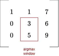
For example, let’s say we’re working with the second pivot at position (1,1). If the largest value is directly below it, the argmax function will return 1, indicating the second row of the window (with the first row being the pivot). However, this index is incorrect, the actual global index should be 1 + 1 = 2. We need to add the offset to account for the rows above the pivot.
def lu_decomposition(A, epsilon: float = 1e-10):

    m, n = A.shape

    # Initialize U as a copy of A, L as identity, and a vector for row swaps
    U = A.copy()
    L = np.eye(n, dtype=float)
    perm = np.arange(n)

    for k in range(n):
        # Partial pivoting: find row with max |U[i, k]| for i >= k
        pivot_row = k + np.argmax(np.abs(U[k:, k]))
        if np.abs(U[pivot_row, k]) < epsilon:
raise np.linalg.LinAlgError("The matrix is singular and cannot be decomposed via LU.")Notice the final check? If the resulting number is zero, or so close to zero that we consider it negligible, this means every number in the column is effectively zero, as there’s no larger absolute value. In this case, the matrix is singular, and we raise the appropriate exception. Recall that a zero column implies linear dependence, which in turn means the matrix has rank less than full. As a result, the matrix is not invertible and is therefore singular.
So far, we’ve only identified the index of the largest number; now it’s time to actually swap the rows. If a row swap is needed (i.e., the pivot index is different from the current row), we swap the corresponding rows in all relevant matrices: \(L\), \(U\), and the array representing \(P\).
When swapping rows in \(U\), we also swap the corresponding entries in \(L\), but only in the columns that have already been filled (i.e columns up to \(k\)). This ensures that \(L\) stays consistent with the new row order of \(U\), so that at the end, \(PA = LU \) still holds. We cannot swap entire rows of \(L\). Think of \(L\) as a logbook of the elimination steps: each column records what happened at that step, and you can only reorder steps that have already occurred. You cannot reorder the future. That would only create wrong results.
def lu_decomposition(A, epsilon: float = 1e-10):

    m, n = A.shape

    # Initialize U as a copy of A, L as identity, and a vector for row swaps
    U = A.copy()
    L = np.eye(n, dtype=float)
    perm = np.arange(n)

    for k in range(n):
        # Partial pivoting: find row with max |U[i, k]| for i >= k
        pivot_row = k + np.argmax(np.abs(U[k:, k]))
        if np.abs(U[pivot_row, k]) < epsilon:
            raise np.linalg.LinAlgError("The matrix is singular and cannot be decomposed via LU.")
if pivot_row != k:
perm[k], perm[pivot_row] = perm[pivot_row], perm[k]
U[[k, pivot_row], :] = U[[pivot_row, k], :]
L[[k, pivot_row], :k] = L[[pivot_row, k], :k]Finally, we eliminate all entries below the pivot. For each row beneath the pivot row, we compute the corresponding multiplier \(l_{ik}\), subtract \(l_{ik}\) times the pivot row from the current row, and store \(l_{ik}\) in the matrix \(L\). To improve efficiency and numerical stability, we skip any row where the entry below the pivot is already zero or sufficiently small (i.e., less than \(\epsilon\)). Now we have the complete code.
def lu_decomposition(A, epsilon: float = 1e-10):

    m, n = A.shape

    # Initialize U as a copy of A, L as identity, and a vector for row swaps
    U = A.copy()
    L = np.eye(n, dtype=float)
    perm = np.arange(n)

    for k in range(n):
        # Partial pivoting: find row with max |U[i, k]| for i >= k
        pivot_row = k + np.argmax(np.abs(U[k:, k]))
        if np.abs(U[pivot_row, k]) < epsilon:
            raise np.linalg.LinAlgError("The matrix is singular and cannot be decomposed via LU.")

        if pivot_row != k:
            perm[k], perm[pivot_row] = perm[pivot_row], perm[k]
            U[[k, pivot_row], :] = U[[pivot_row, k], :]
            L[[k, pivot_row], :k] = L[[pivot_row, k], :k]
# Eliminate below pivot
for i in range(k + 1, n):
factor = U[i, k] / U[k, k]
if abs(U[i, k]) <= epsilon:
continue
L[i, k] = factor
U[i, :] -= factor * U[k, :]
P = np.eye(n)[perm]
return P, L, UDo not forget to return the respective matrices. Note that we construct \(P\) at the very end using the permutation list, essentially by permuting the identity matrix. This way, we create the entire \(P\) in one go.
I left out input-validation code (checking shapes, types, etc.) for educational purposes, as it would clutter the example. That said, in real-world use, you should always bulletproof your code with proper checks and test cases, you never know who will use it.
This is by no means the best possible implementation. For example, it does not distinguish between symmetric, sparse, or banded matrices, cases where certain tricks can make the algorithm much more efficient. In addition, due to Python’s overhead, this code is brutally slow compared to implementations that use LAPACK under the hood, such as those found in libraries like numpy.linalg or scipy.linalg. Whenever possible, you should prefer those libraries instead.
Forward and Backward Substitution
To make practical use of the LU decomposition we have implemented, we need a method for solving the linear system for a given right-hand side vector \(\mathbf{b}\). Fortunately, once \(A\) has been factored, this process is easy.
Starting from
\(
\begin{align}
A\mathbf{x} &= \mathbf{b} \\
LU\mathbf{x} &= \mathbf{b} \\
\end{align}
\)
we introduce an intermediate vector \(\mathbf{c}\) such that
\(L\mathbf{c} = \mathbf{b}\)
followed by
\(U\mathbf{x} = \mathbf{c}\).
Our goal is to compute \(\mathbf{x}\). To do so, we first solve the lower triangular system \(L\mathbf{c}=\mathbf{b}\) using forward substitution. Once \(\mathbf{c}\) is known, we then solve the upper triangular system \(U\mathbf{x}=\mathbf{c}\) using backward substitution.
The key idea behind both methods is that triangular matrices allow us to solve for one variable at a time. In a triangular system, either the first row (lower triangular) or the last row (upper triangular) involves only a single unknown.
Consider the following lower triangular system:
\(Lc = \mathbf{b} \hspace{1cm} \Longleftrightarrow \hspace{1cm} \begin{bmatrix} 1 & 0 & 0 \\ 2 & 3 & 0 \\ 4 & 5 & 6 \end{bmatrix} \begin{bmatrix} c_1 \\ c_2 \\ c_3 \end{bmatrix} = \begin{bmatrix} 1 \\ 9 \\ 8 \end{bmatrix}\)
The first row is already solved for:
\(\begin{align*}1 \cdot c_1 + 0 \cdot c_2 + 0 \cdot c_3 &= 1 \\ c_1 &= 1\end{align*}\)
The second row involves two variables, \(c_1\) and \(c_2\). However, since \(c_1\) is already known, only \(c_2\) remains unknown. We isolate \(c_2\) by moving all known terms to the right-hand side and dividing by the coefficient of \(c_2\).
This process continues row by row. In a lower triangular system, each row depends only on variables from previous rows. As a result, we can work our way forward (top to bottom), substituting previously computed values to solve for the next unknown. Step by step, we build up the solution vector \(\mathbf{c}\).
Backward substitution follows the same principle, but applies to upper triangular matrices. In that case, the last row contains a single unknown, and we work backward (bottom to top), successively substituting known values to solve for the remaining variables.
Forward Substitution Implementation
We’ll start by defining a function with a clear, descriptive name. This function takes three inputs:
- A lower triangular matrix \(L\) (which is not limited to the LU decomposition case, so it may contain non-1 values on the diagonal).
- The right-hand side vector \(\mathbf{b}\).
- A small tolerance value ϵ, which will serve as a threshold for numerical precision, any value smaller than epsilon will be treated as zero.
def forward_substitution(L, b, epsilon: float = 1e-10): Now let’s walk through the logic of the code. We begin by initializing an empty vector \(\mathbf{c}\), which will be filled incrementally as the algorithm progresses. At each iteration, we focus on a single row and solve for the corresponding unknown.
In a given row, one variable is unknown, the one associated with the diagonal entry, while any other variables in that row have already been solved for in previous iterations (or there are none, as in the first row). To account for these known variables, we multiply each one by its corresponding coefficient and sum the results.
In the code, this is done by taking the dot product between the current row of the matrix (up to the \(r\)-th entry, i.e., up to but not including the diagonal) and the portion of the vector \(\mathbf{c}\) that has already been computed. This gives the total contribution of the known variables.
We then subtract this sum from the corresponding entry in \(\mathbf{b}\). Finally, we divide by the diagonal coefficient, the factor in front of the variable we are solving for (labeled div in the code), to obtain the next entry of \(\mathbf{c}\). However, div can’t be zero, if it is, we throw an exception. Finally we return the solution.
def forward_substitution(L, b, epsilon: float = 1e-10):

    c = np.empty_like(b, dtype=np.result_type(L, b, float))

    # Solve rows 0...n‑1
    for r in range(0, n):
        temp = L[r, :r] @ c[:r]
        div = L[r, r]
        if abs(div) < epsilon:
            raise np.linalg.LinAlgError(f"Zero (or near-zero) pivot at row {r}")
        c[r] = (b[r] - temp) / div

return cOnce again, I’ve omitted the input-validation code here, but be sure to include it in your own implementation. Making your code robust and resistant to invalid inputs is always good practice.
The backward substitution code is essentially the same as the forward substitution code, you mainly need to adjust the indices, working from the end of the system instead of the beginning. I won’t write it out explicitly here, but as a helpful tip: in Python, an index of -1 refers to the last element.
Summary
- Each elimination step can be represented by an elimination matrix. Multiplying all of these together yields a single matrix \(E\) such that \(EA=U\). The inverse of \(E\) is \(L\).
- The elimination multipliers appear unchanged in \(L\), falling naturally into their correct positions.
- We use LU decomposition because it makes solving linear systems more efficient. Instead of solving one large system each time the right-hand side \(\mathbf{b}\) changes, we reuse the same factorization and solve two much simpler triangular systems.
- Specifically, we first solve \(L\mathbf{c}=\mathbf{b}\) using forward substitution, and then solve \(U\mathbf{x}=\mathbf{c}\) using backward substitution.